Quick Overview
Prepared by:
To run tutorials in your browser, go to this Binder page.
Note
This tutorial serves as a quick primer to introduce the major (application programming interface) APIs/class in QSDsan and show you its capacities, for detailed instructions on these APIs, please follow the corresponding tutorials in the documentation.
[1]:
import qsdsan as qs
print(f'This tutorial was made with qsdsan v{qs.__version__}.')
This tutorial was made with qsdsan v1.2.0.
[2]:
# Major APIs/classes and related packages of QSDsan shown in the simplified unified modeling language (UML) diagram.
from IPython.display import Image
Image(url='https://lucid.app/publicSegments/view/c8de361f-7292-47e3-8870-d6f668691728/image.png', width=800)
[2]:

[3]:
# Thermodynamics and material flows are handled by `Component` and `WasteStream`
cmps = qs.Components.load_default()
qs.set_thermo(cmps)
cmps.show()
CompiledComponents([S_H2, S_CH4, S_CH3OH, S_Ac, S_Prop, S_F, S_U_Inf, S_U_E, C_B_Subst, C_B_BAP, C_B_UAP, C_U_Inf, X_B_Subst, X_OHO_PHA, X_GAO_PHA, X_PAO_PHA, X_GAO_Gly, X_PAO_Gly, X_OHO, X_AOO, X_NOO, X_AMO, X_PAO, X_MEOLO, X_FO, X_ACO, X_HMO, X_PRO, X_U_Inf, X_U_OHO_E, X_U_PAO_E, X_Ig_ISS, X_MgCO3, X_CaCO3, X_MAP, X_HAP, X_HDP, X_FePO4, X_AlPO4, X_AlOH, X_FeOH, X_PAO_PP_Lo, X_PAO_PP_Hi, S_NH4, S_NO2, S_NO3, S_PO4, S_K, S_Ca, S_Mg, S_CO3, S_N2, S_O2, S_CAT, S_AN, H2O])
[4]:
# Each component is asscociated with many properties
cmps.S_CH4.show(chemical_info=True)
Component: S_CH4 (phase_ref='g')
[Names]  CAS: 74-82-8
         InChI: CH4/h1H4
         InChI_key: VNWKTOKETHGBQD-U...
         common_name: methane
         iupac_name: ('methane',)
         pubchemid: 297
         smiles: C
         formula: CH4
[Groups] Dortmund: <Empty>
         UNIFAC: <Empty>
         PSRK: <Empty>
         NIST: <Empty>
[Data]   MW: 16.042 g/mol
         Tm: 90.75 K
         Tb: 111.65 K
         Tt: 90.698 K
         Tc: 190.56 K
         Pt: 11691 Pa
         Pc: 4.599e+06 Pa
         Vc: 9.86e-05 m^3/mol
         Hf: -74534 J/mol
         S0: 186.3 J/K/mol
         LHV: 8.0257e+05 J/mol
         HHV: 8.9059e+05 J/mol
         Hfus: 940 J/mol
         Sfus: None
         omega: 0.008
         dipole: 0 Debye
         similarity_variable: 0.31167
         iscyclic_aliphatic: 0
         combustion: {'CO2': 1, 'O2'...
Component-specific properties:
[Others] measured_as: COD
         description: Dissolved Methane
         particle_size: Dissolved gas
         degradability: Readily
         organic: True
         i_C: 0.18767 g C/g COD
         i_N: 0 g N/g COD
         i_P: 0 g P/g COD
         i_K: 0 g K/g COD
         i_Mg: 0 g Mg/g COD
         i_Ca: 0 g Ca/g COD
         i_mass: 0.25067 g mass/g COD
         i_charge: 0 mol +/g COD
         i_COD: 1 g COD/g COD
         i_NOD: 0 g NOD/g COD
         f_BOD5_COD: 0
         f_uBOD_COD: 0
         f_Vmass_Totmass: 1
         chem_MW: 16.042
[5]:
# Streams records the flows of each component as well as thermodynamic information
ww = qs.WasteStream.codbased_inf_model('ww', flow_tot=100)
ww.show()
WasteStream: ww
 phase: 'l', T: 298.15 K, P: 101325 Pa
 flow (g/hr): S_F        7.5
              S_U_Inf    3.25
              C_B_Subst  4
              X_B_Subst  22.7
              X_U_Inf    5.58
              X_Ig_ISS   5.23
              S_NH4      2.5
              S_PO4      0.8
              S_K        2.8
              S_Ca       14
              S_Mg       5
              S_CO3      12
              S_N2       1.8
              S_CAT      0.3
              S_AN       1.2
              ...
 WasteStream-specific properties:
  pH         : 7.0
  Alkalinity : 10.0 mg/L
  COD        : 430.0 mg/L
  BOD        : 249.4 mg/L
  TC         : 265.0 mg/L
  TOC        : 137.6 mg/L
  TN         : 40.0 mg/L
  TP         : 10.0 mg/L
  TK         : 28.0 mg/L
 Component concentrations (mg/L):
  S_F          75.0
  S_U_Inf      32.5
  C_B_Subst    40.0
  X_B_Subst    226.7
  X_U_Inf      55.8
  X_Ig_ISS     52.3
  S_NH4        25.0
  S_PO4        8.0
  S_K          28.0
  S_Ca         140.0
  S_Mg         50.0
  S_CO3        120.0
  S_N2         18.0
  S_CAT        3.0
  S_AN         12.0
  ...
[6]:
# Unit operations are modeled as `SanUnit` objects with process and desgin algorithms
print('`qsdsan` now has the following embedded unit operations:\n')
for i in dir(qs.sanunits):
    if not i.startswith('_'):
        print(i)
`qsdsan` now has the following embedded unit operations:

ActivatedSludgeProcess
AnMBR
AnaerobicBaffledReactor
AnaerobicCSTR
AnaerobicDigestion
BeltThickener
BiogasCombustion
BiogenicRefineryCarbonizerBase
BiogenicRefineryControls
BiogenicRefineryGrinder
BiogenicRefineryHHX
BiogenicRefineryHHXdryer
BiogenicRefineryHousing
BiogenicRefineryIonExchange
BiogenicRefineryOHX
BiogenicRefineryPollutionControl
BiogenicRefineryScrewPress
BiogenicRefineryStruvitePrecipitation
CH4E
CHP
CSTR
ComponentSplitter
Copier
CropApplication
Decay
DryingBed
DynamicInfluent
EcoSanAerobic
EcoSanAnaerobic
EcoSanAnoxic
EcoSanBioCost
EcoSanECR
EcoSanMBR
EcoSanPrimary
EcoSanSolar
EcoSanSystem
ElectrochemicalCell
Excretion
FakeSplitter
FlatBottomCircularClarifier
H2E
HXprocess
HXutility
HydraulicDelay
IdealClarifier
InternalCirculationRx
Lagoon
LiquidTreatmentBed
LumpedCost
MURT
MixTank
Mixer
PitLatrine
PolishingFilter
Pump
ReclaimerECR
ReclaimerHousing
ReclaimerIonExchange
ReclaimerSolar
ReclaimerSystem
ReclaimerUltrafiltration
ReversedSplitter
SBR
Sampler
Screening
Sedimentation
SepticTank
SludgeCentrifuge
SludgeDigester
SludgePasteurization
SludgeSeparator
SludgeThickening
Splitter
StorageTank
Tank
Toilet
Trucking
UDDT
WWTpump
wwtpump
[7]:
# Dynamic simulation is realized through the `Process` class
cmps = qs.processes.create_asm1_cmps(set_thermo=True)
asm1 = qs.processes.ASM1(Y_A=0.24, Y_H=0.67, f_P=0.08, i_XB=0.08, i_XP=0.06,
                        mu_H=4.0, K_S=10.0, K_O_H=0.2, K_NO=0.5, b_H=0.3,
                        eta_g=0.8, eta_h=0.8, k_h=3.0, K_X=0.1, mu_A=0.5,
                        K_NH=1.0, b_A=0.05, K_O_A=0.4, k_a=0.05, fr_SS_COD=0.75)
asm1.show()
ASM1([aero_growth_hetero, anox_growth_hetero, aero_growth_auto, decay_hetero, decay_auto, ammonification, hydrolysis, hydrolysis_N])
[8]:
asm1.aero_growth_hetero
Process: aero_growth_hetero
[stoichiometry]      S_S: -1.0/Y_H
                     X_BH: 1.00
                     S_O: 1.0*(Y_H - 1.0)/Y_H
                     S_NH: -0.0800
[reference]          X_BH
[rate equation]      S_NH*S_O*S_S*X_BH*mu_H/((K_N...
[parameters]         Y_H: 0.67
                     Y_A: 0.24
                     f_P: 0.08
                     mu_H: 4
                     K_S: 10
                     K_O_H: 0.2
                     K_NO: 0.5
                     b_H: 0.3
                     mu_A: 0.5
                     K_NH: 1
                     K_O_A: 0.4
                     b_A: 0.05
                     eta_g: 0.8
                     k_a: 0.05
                     k_h: 3
                     K_X: 0.1
                     eta_h: 0.8
[dynamic parameters]
[9]:
print(asm1.rate_equations) # looks nicer in the dark mode in readthedocs than just `asm1.rate_equations`
                                         rate_equation
aero_growth_hetero  4.0*S_NH*S_O*S_S*X_BH/((S_NH + ...
anox_growth_hetero  0.64*S_NH*S_NO*S_S*X_BH/((S_NH ...
aero_growth_auto    0.5*S_NH*S_O*X_BA/((S_NH + 1.0)...
decay_hetero                                  0.3*X_BH
decay_auto                                   0.05*X_BA
ammonification                          0.05*S_ND*X_BH
hydrolysis          3.0*X_BH*X_S*(0.16*S_NO/((S_NO ...
hydrolysis_N        3.0*X_BH*X_ND*(0.16*S_NO/((S_NO...
[10]:
# Upon simulation, you can easily retrive information related to a specific unit
# `exposan` contains systems developed using `qsdsan`,
# find more about the following exemplary system here:
# https://github.com/QSD-Group/EXPOsan/tree/main/exposan/bwaise
from exposan import bwaise as bw
# Each blue error in the diagram is a stream
bw.load()
[11]:
# The `result` function can show the simulated results
print(bw.A2.results())
Pit latrine                                      Units       A2
Design              Number of users per toilet               16
                    Parallel toilets                   2.85e+04
                    Emptying period                 yr      0.8
                    Single pit volume               m3     3.66
                    Single pit area                 m2      0.8
                    Single pit depth                 m     4.57
                    Cement                          kg    2e+07
                    Sand                            kg 9.05e+07
                    Gravel                          kg 3.65e+07
                    Brick                           kg 6.47e+06
                    Plastic                         kg 2.88e+05
                    Steel                           kg 9.58e+05
                    Wood                            m3 5.42e+03
                    Excavation                      m3 1.04e+05
Purchase cost       Total toilets                  USD 1.28e+07
Total purchase cost                                USD 1.28e+07
Utility cost                                    USD/hr        0
Additional OPEX                                 USD/hr     73.1
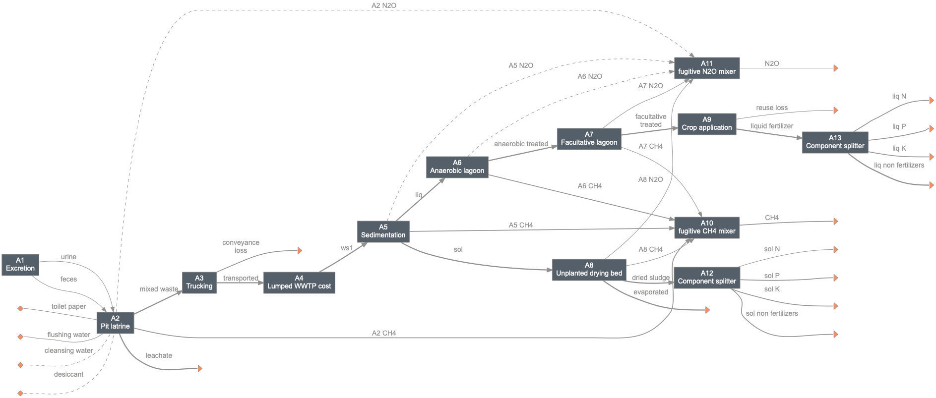
[12]:
# You can create systems by linking different units
bw.sysA.diagram()
[13]:
# `TEA` and `LCA` classes are used for techno-economic analysis and life cycle assessment
c = qs.currency
print('For sysA in the Bwaise study:\n')
for attr in ('NPV', 'EAC', 'CAPEX', 'AOC', 'sales', 'net_earnings'):
    uom = c if attr in ('NPV', 'CAPEX') else (c+('/yr'))
    print(f'{attr} is {getattr(bw.teaA, attr):,.0f} {uom}')
For sysA in the Bwaise study:

NPV is -42,012,332 USD
EAC is 6,706,241 USD/yr
CAPEX is 31,421,918 USD
AOC is 1,844,585 USD/yr
sales is 206,017 USD/yr
net_earnings is -1,638,568 USD/yr
[14]:
bw.lcaA
LCA: sysA (lifetime 8 yr)
Impacts:
                           Construction  Transportation   Stream   Others    Total
GlobalWarming (kg CO2-eq)      3.13e+07        9.57e+05 1.82e+08 5.19e+04 2.14e+08
[15]:
# Finally, uncertainty and sensitivity analyses are handled by `Model`
bw.modelA # below shows the uncertainty parameters
Finally, qsdsan also has a stats module with many global sensitivity analyses and visualization tools to generate quick and nice figures.
Back to top