Uncertainty and Sensitivity Analyses¶
Click the badge below to try this tutorial interactively in your browser:
![]()
You can also run this tutorial inGoogle Colab. It takes a one-time setup per session: follow theColab instructions.
Prepared by:
Learning objectives. After this tutorial, you will be able to:
Define
ParameterandMetricobjects on aModelRun Monte Carlo uncertainty analysis
Perform sensitivity analysis (rank correlation, Morris, FAST/Sobol)
Covered topics:
Model, Parameter, and Metric
Perform Uncertainty and Sensitivity Analyses
Companion video. A walkthrough of this tutorial is available on YouTube, presented by Hannah Lohman. Recorded against
QSDsanv1.2.0. The concepts still apply, but if the code on screen differs from this notebook, follow the notebook.
Setup¶
Import QSDsan and confirm the installed version.
[1]:
import qsdsan as qs
print(f'This tutorial was made with qsdsan v{qs.__version__}.')
This tutorial was made with qsdsan v1.5.3.
1. Model, Parameter, and Metric¶
To perform uncertainty and sensitivity analyses, we wrap a System in a Model, then attach Parameter objects (the uncertain inputs) and Metric objects (the outputs we care about).
1.1. Build the system with TEA and LCA¶
We reuse the aerobic activated-sludge plant from the 7. TEA and 8. LCA tutorials (4,000 m³/d, COD ≈ 430 mg/L), packaged for convenience as qsdsan.utils.create_example_treatment_systems. That tutorial pair walks through how the plant, its TEA, and its LCA are built; here we just recap the setup before turning the knobs.
The LCA registries (indicators, items, construction, transportation) are scoped to the active flowsheet, so we work in a dedicated flowsheet to keep this tutorial isolated from anything you may have loaded elsewhere.
[2]:
from qsdsan import Model
from qsdsan.utils import create_example_treatment_systems

# Dedicated flowsheet keeps this tutorial's LCA registries isolated
qs.main_flowsheet.set_flowsheet('uncertainty_demo')

# Impact indicator lives in the active flowsheet, so (re)define it here
qs.ImpactIndicator('GlobalWarming', alias='GWP', unit='kg CO2-eq')

# Aerobic plant from 7_TEA / 8_LCA (we ignore the anaerobic one for this tutorial)
aer_sys, _ = create_example_treatment_systems()
aer = aer_sys.units[0]
aer_sys.simulate()
aer_sys.diagram()

[3]:
# TEA: revenue comes from a treatment fee on the influent.
# A negative stream price means the plant is paid to take the wastewater
# (so revenue = -price * mass flow); see the 7_TEA tutorial for context.
ww = aer.ins[0]
ww.price = -0.0006              # USD/kg (~$0.60/m3 treatment fee)
qs.PowerUtility.price = 0.08    # USD/kWh
tea = qs.TEA(aer_sys, discount_rate=0.05, lifetime=20)
[4]:
# LCA: a little concrete and steel for the reactor (Construction items),
# plus electricity as an "other" activity that tracks the simulation.
Concrete = qs.ImpactItem('Concrete', functional_unit='m3', GWP=300.)
Steel    = qs.ImpactItem('Steel',    functional_unit='kg', GWP=2.)
electricity = qs.ImpactItem('electricity', functional_unit='kWh', GWP=0.6)

aer.construction = [
    qs.Construction(linked_unit=aer, item=Concrete, quantity=300,
                    quantity_unit='m3', lifetime=30),
    qs.Construction(linked_unit=aer, item=Steel,    quantity=30000,
                    quantity_unit='kg', lifetime=30),
]
[5]:
lifetime = 20
lca = qs.LCA(system=aer_sys, lifetime=lifetime,
             electricity=lambda: aer.power_utility.rate * 24 * 365 * lifetime,
             simulate_system=False)
Declaring default materials. Here we attach Construction objects to an existing unit instance because the aerobic plant did not declare any built-in construction materials. For new unit classes that always need certain materials, declare them once as a class-level _construction_specs tuple instead; see § 4 of 8. LCA for the canonical pattern.
1.2. Create a system model and add uncertainty parameters and metrics¶
The Model class wraps a System and exposes the parameter and metric decorators we use to declare uncertain inputs and tracked outputs.
[6]:
model = Model(aer_sys)
Uncertainty parameters can be added with model.parameter. For this plant we add six:
Treatment fee charged for influent (TEA)
Electricity price (TEA)
Installed plant capital (TEA)
Steel GWP characterization factor (LCA)
Electricity GWP characterization factor (LCA)
Fraction of substrate oxidized,
X_oxid(couples to both): it changes the oxygen demand and so the electricity consumption
[7]:
# We use the package `chaospy` to create the distributions
from chaospy import distributions as shape
[8]:
# There are several ways to register parameters; the decorator form below is the most common.
param = model.parameter

# A treatment fee that varies between $0.30 and $1.00 per m3 of influent.
# `element` labels which part of the system the parameter belongs to (free-form string or object);
# `kind='isolated'` means the value is read at evaluation time but does not require resimulation
# (only `_cost` reads the wastewater price, not `_run`).
dist = shape.Uniform(lower=0.30, upper=1.00)
@param(name='Treatment fee', element='TEA', kind='isolated',
       units='USD/m3', baseline=0.60, distribution=dist)
def set_fee(fee_per_m3):
    ww.price = -fee_per_m3 / 1000   # USD/kg, negative = revenue
[9]:
# The same `parameter` API also accepts a `setter=` callable, which is handy when the
# setter is a one-liner or comes from elsewhere.
baseline = qs.PowerUtility.price
dist = shape.Triangle(lower=baseline*0.75, midpoint=baseline, upper=baseline*1.25)

def set_e_price(p):
    qs.PowerUtility.price = p

param(setter=set_e_price, name='Electricity price', kind='isolated', element='TEA',
      units='USD/kWh', baseline=baseline, distribution=dist)
[9]:
<Parameter: [TEA] Electricity price (USD/kWh)>
[10]:
# LCA characterization factors. They feed only the LCA, so `kind='isolated'`.
baseline = Steel.CFs['GlobalWarming']
dist = shape.Uniform(lower=baseline*0.9, upper=baseline*1.5)
@param(name='Steel GWP', element='LCA', kind='isolated',
       units='kg CO2-eq/kg', baseline=baseline, distribution=dist)
def set_steel_GWP(cf):
    Steel.CFs['GlobalWarming'] = cf

baseline = electricity.CFs['GlobalWarming']
dist = shape.Uniform(lower=baseline*0.7, upper=baseline*1.3)
@param(name='Electricity GWP', element='LCA', kind='isolated',
       units='kg CO2-eq/kWh', baseline=baseline, distribution=dist)
def set_e_GWP(cf):
    electricity.CFs['GlobalWarming'] = cf
[11]:
# Installed plant capital. Cost only, so still `kind='isolated'`.
baseline = aer.plant_capital
dist = shape.Triangle(lower=baseline*0.8, midpoint=baseline, upper=baseline*1.2)
@param(name='Plant capital', element=aer, kind='isolated',
       units='USD', baseline=baseline, distribution=dist)
def set_plant_capital(c):
    aer.plant_capital = c

# Fraction of substrate oxidized. This one feeds `_run` (it changes the O2 demand
# and therefore the electricity draw), so it must be `kind='coupled'` to trigger a resimulation.
baseline = aer.X_oxid
dist = shape.Uniform(lower=0.85, upper=0.99)
@param(name='X_oxid', element=aer, kind='coupled',
       units='-', baseline=baseline, distribution=dist)
def set_X_oxid(x):
    aer.X_oxid = x
[12]:
# Metrics. As with `parameter`, both decorator and functional forms work.
metric = model.metric

@metric(name='Net earnings', units='USD/yr', element='TEA')
def get_net_earnings():
    return tea.net_earnings

# In 8_LCA we switched to `get_total_impacts(time_frame='yr')`, which returns
# annual impacts directly and updates the unit suffix on save_report tables.
def get_annual_GWP():
    return lca.get_total_impacts(time_frame='yr')['GlobalWarming']
metric(getter=get_annual_GWP, name='GWP', units='kg CO2-eq/yr', element='LCA')
[12]:
<Indicator: [LCA] GWP (kg CO2-eq/yr)>
[13]:
model.show()
Model:
parameters: TEA - Treatment fee [USD/m3]
            TEA - Electricity price [USD/kWh]
            LCA - Steel GWP [kg CO2-eq/kg]
            LCA - Electricity GWP [kg CO2-eq/kWh]
            Aerobic plant-Aer - Plant capital [USD]
            Aerobic plant-Aer - X oxid [-]
indicators: TEA - Net earnings [USD/yr]
            LCA - GWP [kg CO2-eq/yr]
2. Perform uncertainty and sensitivity analyses¶
2.1. Uncertainty analysis¶
[14]:
# Sample the joint parameter space with Latin hypercube (`rule='L'`).
import numpy as np
np.random.seed(3221)   # for reproducibility

samples = model.sample(N=100, rule='L')
model.load_samples(samples)
[15]:
# Run the 100 simulations
model.evaluate()
[16]:
# Parameter values and metric results are stored in `model.table`
model.table
[16]:
| Element | TEA | LCA | Aerobic plant-Aer | TEA | LCA | |||
|---|---|---|---|---|---|---|---|---|
| Variable | Treatment fee [USD/m3] | Electricity price [USD/kWh] | Steel GWP [kg CO2-eq/kg] | Electricity GWP [kg CO2-eq/kWh] | Plant capital [USD] | X oxid [-] | Net earnings [USD/yr] | GWP [kg CO2-eq/yr] |
| 0 | 0.571 | 0.083 | 1.93 | 0.647 | 5.16e+06 | 0.967 | 7.95e+05 | 2.04e+05 |
| 1 | 0.701 | 0.0737 | 2.66 | 0.458 | 5.65e+06 | 0.897 | 9.89e+05 | 1.38e+05 |
| 2 | 0.452 | 0.0688 | 2.64 | 0.71 | 5.04e+06 | 0.905 | 6.27e+05 | 2.1e+05 |
| 3 | 0.553 | 0.0702 | 2.46 | 0.577 | 4.31e+06 | 0.919 | 7.73e+05 | 1.75e+05 |
| 4 | 0.509 | 0.0903 | 2.34 | 0.724 | 5.28e+06 | 0.977 | 7.01e+05 | 2.3e+05 |
| ... | ... | ... | ... | ... | ... | ... | ... | ... |
| 95 | 0.757 | 0.0679 | 2.13 | 0.694 | 4.58e+06 | 0.88 | 1.07e+06 | 1.99e+05 |
| 96 | 0.346 | 0.0864 | 2.95 | 0.684 | 5.1e+06 | 0.869 | 4.68e+05 | 1.96e+05 |
| 97 | 0.966 | 0.0706 | 2.7 | 0.554 | 5.57e+06 | 0.903 | 1.38e+06 | 1.66e+05 |
| 98 | 0.543 | 0.0762 | 2.95 | 0.533 | 5.41e+06 | 0.954 | 7.57e+05 | 1.69e+05 |
| 99 | 0.694 | 0.0793 | 2.04 | 0.426 | 5.05e+06 | 0.974 | 9.74e+05 | 1.38e+05 |
100 rows × 8 columns
Optional: result organization and exporting (click to expand)
You can split the results table into parameters, results, and percentiles and write them to Excel:
import pandas as pd
def organize_results(model, path):
    idx = len(model.parameters)
    parameters = model.table.iloc[:, :idx]
    results = model.table.iloc[:, idx:]
    percentiles = results.quantile([0, 0.05, 0.25, 0.5, 0.75, 0.95, 1])
    with pd.ExcelWriter(path) as writer:
        parameters.to_excel(writer, sheet_name='Parameters')
        results.to_excel(writer, sheet_name='Results')
        percentiles.to_excel(writer, sheet_name='Percentiles')

organize_results(model, 'example_model.xlsx')
For convenience, the qsdsan.stats analysis functions (get_correlations, morris_analysis, …) all take a file= argument that writes results straight to Excel.
QSDsan ships a small qsdsan.stats module that wraps SALib (sensitivity analysis) and seaborn (plotting) for the most common uncertainty and sensitivity workflows; the rest of this tutorial uses it. See the stats module API page for the full list of analysis and plotting functions, along with their signatures and worked examples.
[17]:
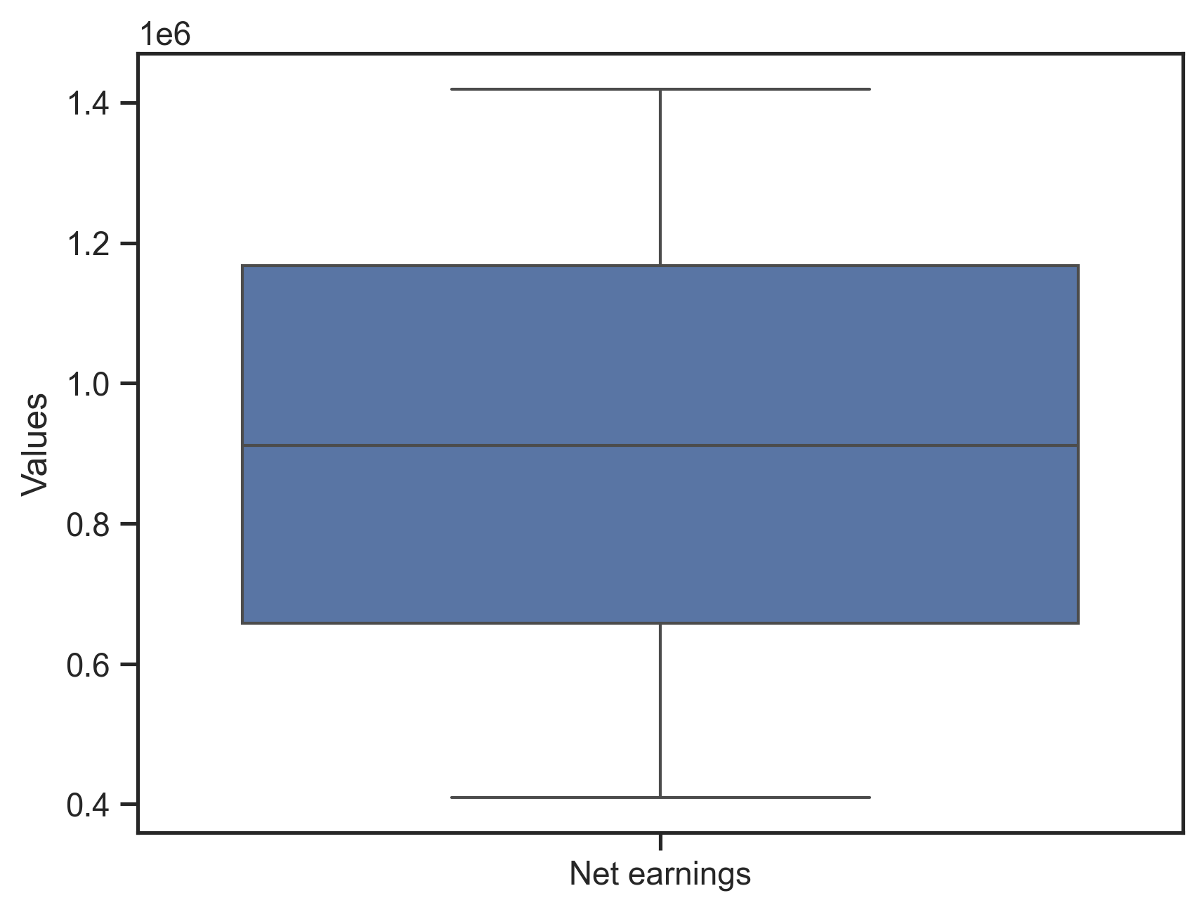
# Marginal distribution of the TEA metric
fig, ax = qs.stats.plot_uncertainties(model, x_axis=model.metrics[0])
fig
[17]:
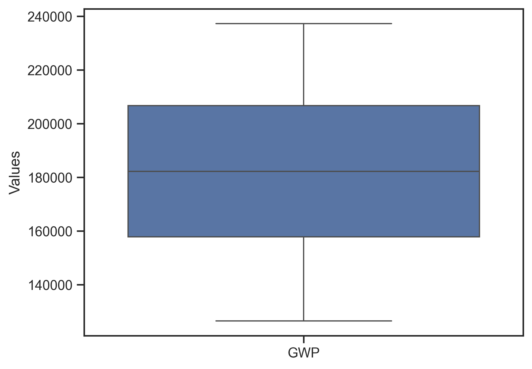
[18]:
# Marginal distribution of the LCA metric (drawn separately so it gets its own y-scale)
fig, ax = qs.stats.plot_uncertainties(model, x_axis=model.metrics[1])
fig
[18]:
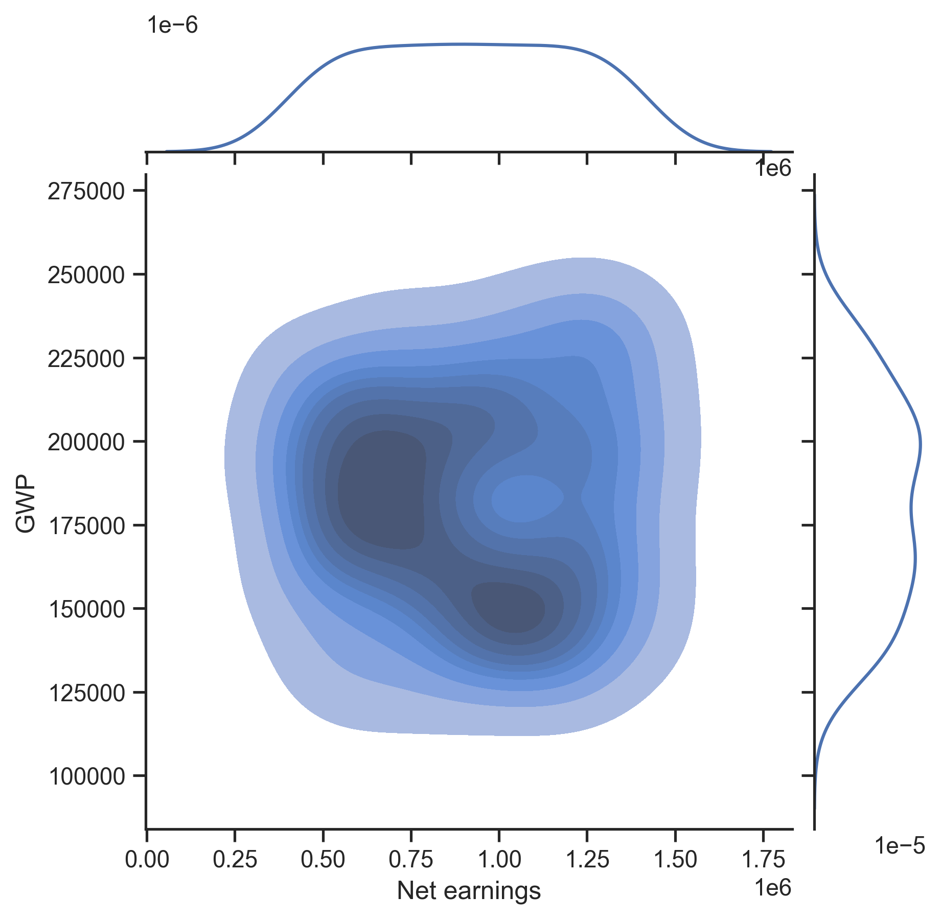
[19]:
# 2-D KDE shows the joint distribution
fig, ax = qs.stats.plot_uncertainties(model, x_axis=model.metrics[0], y_axis=model.metrics[1],
                                      kind='kde-kde', center_kws={'fill': True})
fig
[19]:
2.2. Sensitivity analysis¶
qsdsan.stats exposes four families of sensitivity methods, each paired with a plot_* companion:
Method |
Function |
Plot |
Notes |
|---|---|---|---|
Rank correlation (Spearman / Pearson / Kendall / KS) |
|
|
cheap; reuses the Monte Carlo table from § 2.1. |
Elementary effects (Morris) |
|
|
one-at-a-time screening with its own sampler. |
Fourier amplitude (eFAST / RBD-FAST) |
|
|
variance-based, single-index. |
Sobol indices |
|
|
variance-based, first-order + total. |
Each function and each plot_* companion accepts a file= argument that writes results to Excel. See the stats module API page for full signatures and the worked FAST/Sobol examples we skip below.
2.2.1. Rank correlation¶
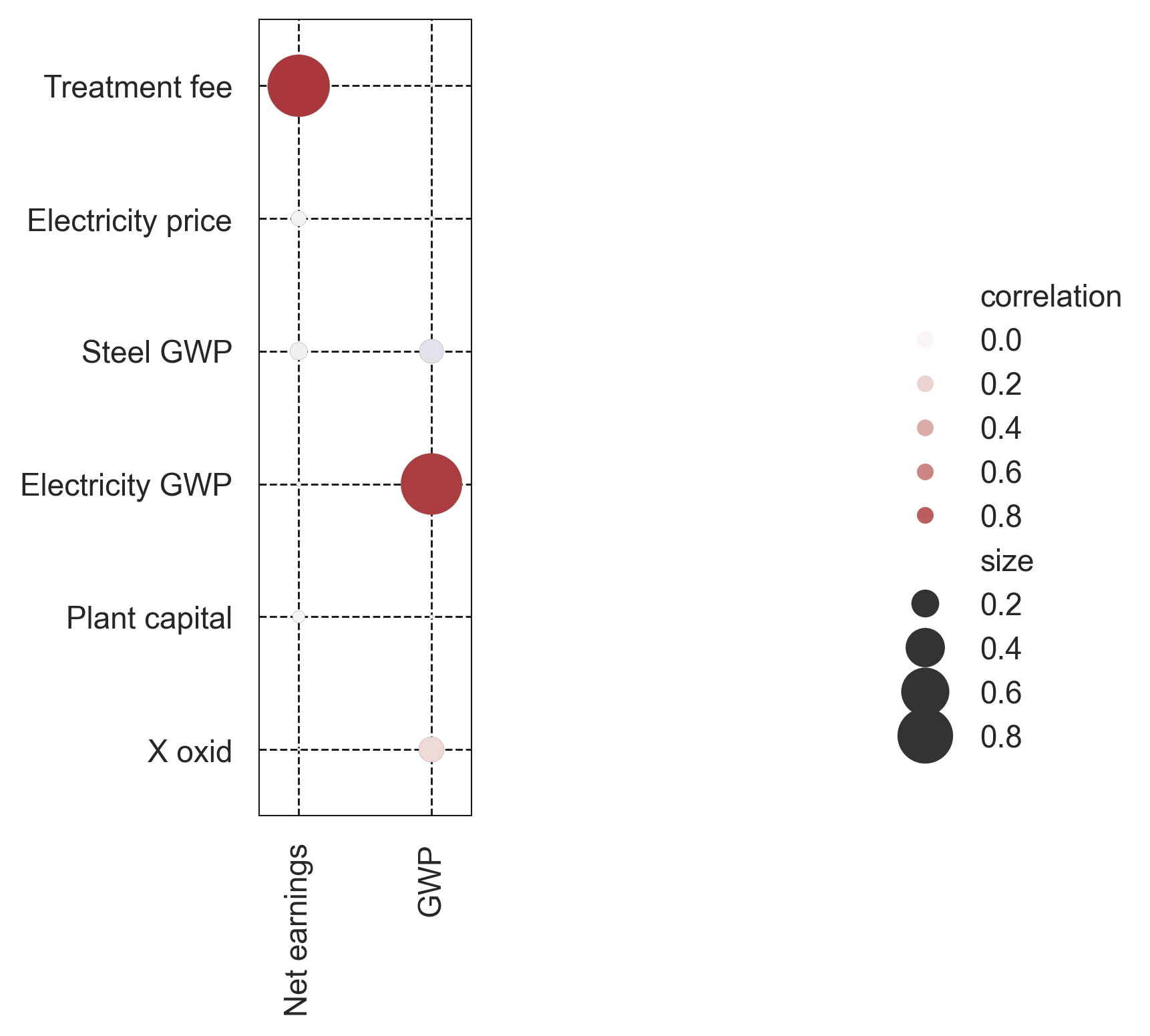
Rank correlation reuses the Monte Carlo samples we already generated, so it is the cheapest (i.e., uses the least additional computational resources) screening tool. get_correlations returns two multi-indexed DataFrames: the correlation coefficients and their p-values.
[20]:
# `r_df` and `p_df` are dataframes containing the correlation coefficients and p-values.
r_df, p_df = qs.stats.get_correlations(model, kind='Spearman')
r_df.round(2)
[20]:
| Element | TEA | LCA | |
|---|---|---|---|
| Input y | Net earnings [USD/yr] | GWP [kg CO2-eq/yr] | |
| Element | Input x | ||
| TEA | Treatment fee [USD/m3] | 1 | 0 |
| Electricity price [USD/kWh] | -0.06 | -0.01 | |
| LCA | Steel GWP [kg CO2-eq/kg] | -0.08 | -0.15 |
| Electricity GWP [kg CO2-eq/kWh] | 0.01 | 0.97 | |
| Aerobic plant-Aer | Plant capital [USD] | -0.04 | 0 |
| X oxid [-] | 0 | 0.16 |
[21]:
p_df.round(3)
[21]:
| Element | TEA | LCA | |
|---|---|---|---|
| Input y | Net earnings [USD/yr] | GWP [kg CO2-eq/yr] | |
| Element | Input x | ||
| TEA | Treatment fee [USD/m3] | 0 | 0.985 |
| Electricity price [USD/kWh] | 0.546 | 0.954 | |
| LCA | Steel GWP [kg CO2-eq/kg] | 0.432 | 0.132 |
| Electricity GWP [kg CO2-eq/kWh] | 0.954 | 0 | |
| Aerobic plant-Aer | Plant capital [USD] | 0.698 | 0.967 |
| X oxid [-] | 0.985 | 0.102 |
[22]:
# The bubble chart makes the result much easier to read at a glance.
fig, ax = qs.stats.plot_correlations(r_df)
fig
[22]:
2.2.2. Elementary effects (Morris)¶
Morris One-at-A-Time screening estimates each parameter’s mean absolute elementary effect (μ*) and the standard deviation of those effects (σ). Parameters with high μ* are influential; parameters with high σ relative to μ* have nonlinear or interaction effects. Morris uses its own sampling design, so we generate fresh samples and re-evaluate before calling morris_analysis.
[23]:
import matplotlib.pyplot as plt

inputs = qs.stats.define_inputs(model)
samples = qs.stats.generate_samples(inputs, kind='Morris', N=10, seed=554)
model.load_samples(samples)
model.evaluate()
morris_dct = qs.stats.morris_analysis(model, inputs, seed=554, nan_policy='fill_mean')

# One panel per metric so each gets its own (mu*, sigma) scale
fig, axes = plt.subplots(1, 2, figsize=(12, 4.5))
for ax, m in zip(axes, model.metrics):
    qs.stats.plot_morris_results(morris_dct, metric=m, ax=ax, label_kind='name')
    ax.set_title(m.name)
fig.tight_layout()
fig
[23]:
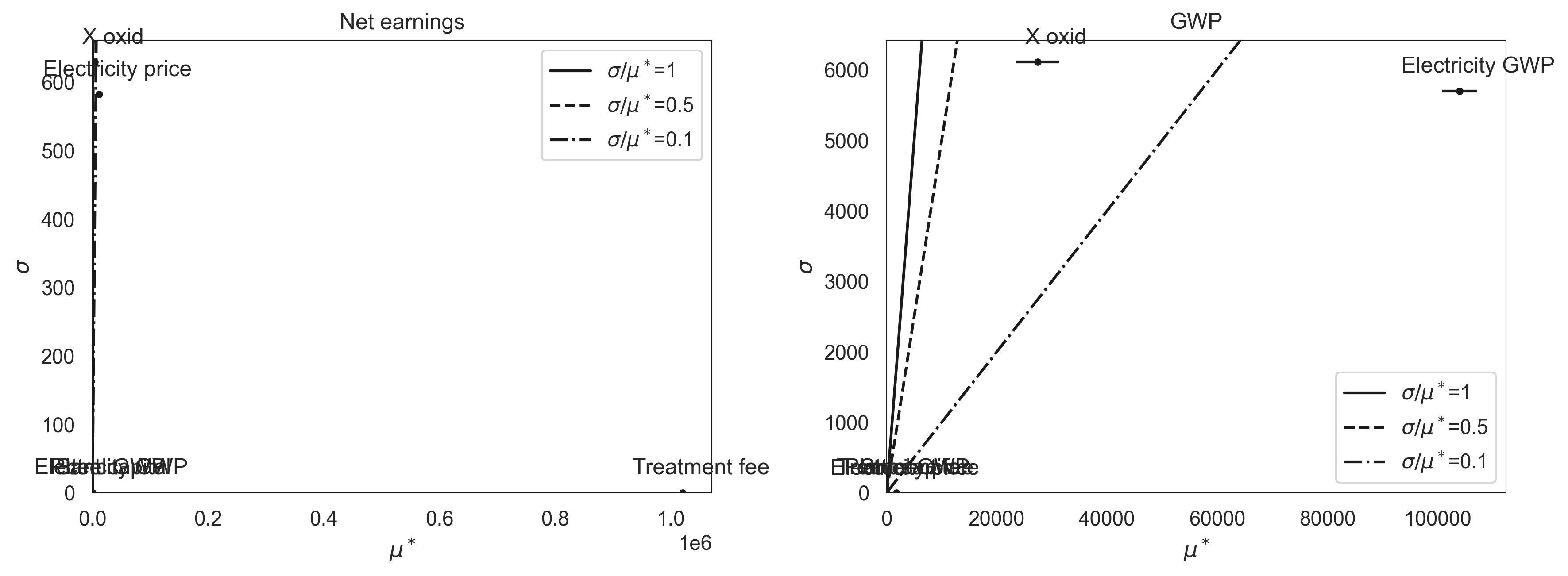
The Net earnings panel is dominated by the treatment fee (consistent with the Spearman result above), so the other five parameters collapse near the origin. The GWP panel is more informative: the electricity CF has the largest mean effect; X_oxid sits high on σ relative to μ*, signalling a nonlinear or interaction-driven contribution (it changes both the oxygen demand and the electricity draw it feeds into).
2.2.3. Variance-based methods (FAST and Sobol)¶
fast_analysis and sobol_analysis follow the same shape as Morris: generate a method-specific sample with generate_samples, evaluate the model, then call the analysis function. They are more expensive (Sobol especially) but partition the output variance into first-order and (for Sobol) total-order indices that capture interactions. See the worked examples on the stats module API page.
↑ Back to top