Dynamic Simulation

Click the badge below to try this tutorial interactively in your browser:

You can also run this tutorial inGoogle Colab. It takes a one-time setup per session: follow theColab instructions.

• Prepared by:

  • Joy Zhang

• Learning objectives. After this tutorial, you will be able to:

  • Set up and run a dynamic simulation

  • Manage state variables and time-series outputs

  • Save and inspect dynamic results

• Prerequisites: 10. Process

• Covered topics:

  • 1. Understanding dynamic simulation with QSDsan

  • 2. Writing a dynamic SanUnit

  • 3. Other convenient features

Companion video. A walkthrough of this tutorial is available on YouTube, presented by Yalin Li. Recorded against QSDsan v1.3.1. The concepts still apply, but if the code on screen differs from this notebook, follow the notebook.

Setup

Import QSDsan and confirm the installed version.

import qsdsan as qs, exposan
print(f'This tutorial was made with qsdsan v{qs.__version__} and exposan v{exposan.__version__}')

This tutorial was made with qsdsan v1.5.3 and exposan v1.5.3

1. Understanding dynamic simulation with QSDsan

From previous tutorials, we’ve covered how to use QSDsan’s SanUnit and WasteStream classes to model the mass/energy flows throughout a system. You may have noticed, the simulation results generated by SanUnit._run are static, i.e., they don’t carry time-related information.

In this tutorial, we will learn about the dynamic simulation features in QSDsan. First we will focus on performing dynamic simulations with an existing system to understand the basics. Then we’ll go over how to implement your own algorithms for dynamic simulations.

1.1. An example system

Let’s use Benchmark Simulation Model no.1 (BSM1) as an example. BSM1 describes an activated sludge treatment process that can be commonly found in conventional wastewater treatment facilities. It uses the same activated-sludge layout (two anoxic tanks, three aerated tanks, and a clarifier with two recycles) built and illustrated in 6. System; here we load the full implementation, with process models, from EXPOsan.

1.1.1. Running dynamic simulation

# Let's load the BSM1 system first
from exposan import bsm1
bsm1.load()
sys = bsm1.sys

# The BSM1 system is composed of 5 CSTRs in series,
# followed by a flat-bottom circular clarifier.
# sys.units
sys.diagram()

# If we try to simulate it like we'd do for a "static" system
sys.simulate()

---------------------------------------------------------------------------
TypeError                                 Traceback (most recent call last)
Cell In[3], line 2
      1 # If we try to simulate it like we'd do for a "static" system
----> 2 sys.simulate()

File ~\Documents\Coding\QSDsan-platform\.venv\Lib\site-packages\biosteam\_system.py:3374, in System.simulate(self, update_configuration, units, design_and_cost, **kwargs)
   3354 def simulate(self, update_configuration: Optional[bool]=None, units=None,
   3355              design_and_cost=None, **kwargs):
   3356     """
   3357     If system is dynamic, run the system dynamically. Otherwise, converge 
   3358     the path of unit operations to steady state. After running/converging 
   (...)   3372         
   3373     """
-> 3374     with self.flowsheet:
   3375         specifications = self._specifications
   3376         if specifications and not self._running_specifications:

File ~\Documents\Coding\QSDsan-platform\.venv\Lib\site-packages\biosteam\_flowsheet.py:120, in Flowsheet.__exit__(self, type, exception, traceback)
    118 def __exit__(self, type, exception, traceback):
    119     main_flowsheet.set_flowsheet(self._temporary_stack.pop())
--> 120     if exception: raise exception

File ~\Documents\Coding\QSDsan-platform\.venv\Lib\site-packages\biosteam\_system.py:3418, in System.simulate(self, update_configuration, units, design_and_cost, **kwargs)
   3416 self._setup(update_configuration, units)
   3417 if self.isdynamic:
-> 3418     outputs = self.dynamic_run(**kwargs)
   3419     if design_and_cost: self._summary()
   3420 else:

File ~\Documents\Coding\QSDsan-platform\.venv\Lib\site-packages\biosteam\_system.py:3513, in System.dynamic_run(self, **dynsim_kwargs)
   3511 # Integrate
   3512 self.dynsim_kwargs['print_t'] = print_t # self.dynsim_kwargs might be reset by `state_reset_hook`
-> 3513 self.scope.sol = sol = solve_ivp(fun=self.DAE, y0=y0, **dk_cp)
   3514 if print_msg:
   3515     if sol.status == 0:

TypeError: solve_ivp() missing 1 required positional argument: 't_span'

We run into this error because QSDsan (essentially biosteam in the background) considers this system dynamic, and additional arguments are required for simulate to work.

# We can verify that by
sys.isdynamic

True

# This is because the system contains at least one dynamic SanUnit
{u: u.isdynamic for u in sys.units}

{<CSTR: A1>: True,
 <CSTR: A2>: True,
 <CSTR: O1>: True,
 <CSTR: O2>: True,
 <CSTR: O3>: True,
 <FlatBottomCircularClarifier: C1>: True}

# If we disable dynamic simulation, then `simulate` would work as usual
sys.isdynamic = False
sys.simulate()
sys.show()

System: bsm1_sys
Highest convergence error among components in recycle
streams {C1-1, O3-0} after 1 loops:
- flow rate   1.46e-11 kmol/hr (2.7e-14%)
- temperature 0.00e+00 K (0%)
ins...
[0] wastewater
    phase: 'l', T: 293.15 K, P: 101325 Pa
    flow (kmol/hr): S_I   23.1
                    S_S   53.4
                    X_I   39.4
                    X_S   155
                    X_BH  21.7
                    S_NH  1.73
                    S_ND  5.34
                    ...   4.26e+04
outs...
[0] effluent
    phase: 'l', T: 293.15 K, P: 101325 Pa
    flow (kmol/hr): S_I   22.6
                    S_S   52.3
                    X_I   38.5
                    X_S   152
                    X_BH  21.2
                    S_NH  1.7
                    S_ND  5.23
                    ...   4.17e+04
[1] WAS
    phase: 'l', T: 293.15 K, P: 101325 Pa
    flow (kmol/hr): S_I   0.481
                    S_S   1.11
                    X_I   0.821
                    X_S   3.25
                    X_BH  0.452
                    S_NH  0.0361
                    S_ND  0.111
                    ...   888

To perform a dynamic simulation of the system, we need to provide at least one additional keyword argument, i.e., t_span, as suggested in the error message. t_span is a 2-tuple indicating the simulation period.

Note: Whether t_span = (0,10) means 0-10 days or 0-10 hours/minutes/months depends entirely on units of the parameters in the system’s ODEs. For BSM1, it’d mean 0-10 days because all parameters in the ODEs express time in the unit of “day”.

Other often-used keyword arguments include:

• t_eval: a 1d array to specify the output time points

• method: a string specifying the ordinary differential equation (ODE) solver

• atol and rtol: the absolute and relative error tolerances the solver holds each step to; tighten them (smaller values) if a trajectory looks under-resolved or jagged, or loosen them to trade accuracy for speed

• state_reset_hook: controls what happens to the system’s dynamic state before integration starts. Common values:

  • 'reset_cache' — clear the compiled DAE plus every unit’s and stream’s _state / _dstate, then re-initialize from the static-converged design. Use this when you want each sys.simulate(...) call to behave like a fresh first run (e.g., after changing influent characteristics, kinetic parameters, or unit sizes between simulations). It’s the safe default when you’re not sure.

  • 'clear_state' — lighter-weight: zero out unit and stream state arrays but keep the compiled DAE. Useful when only the initial conditions changed.

  • None (default) — leave existing state intact. The next simulation resumes from wherever the previous one left off — useful for stitching successive time windows together, or for warm-starting from a converged state.

t_span, t_eval, method, atol, and rtol are essentially passed to scipy.integrate.solve_ivp as keyword arguments. See the System.dynamic_run documentation for a complete list of keyword arguments (it also accepts print_msg=True, which prints the solver’s completion or failure message, useful when a run does not finish). You may notice that scipy.integrate.solve_ivp also requires input of fun (i.e., the ODEs) and y0 (i.e., the initial condition); we’ll come back to how System.simulate automates the compilation of these inputs in §2.1.

Tip: For systems that are expected to converge to some sort of “steady state”, it is usually faster to simulate with implicit ODE solvers (e.g., method = BDF or method = LSODA) than with explicit ones. If one solver fails to complete integration through the entire specified simulation period, always try with alternative ones. See scipy.integrate.solve_ivp for the full list of methods and guidance on choosing among them.

# Let's try simulating the BSM1 system from day 0 to day 50 in the dynamic mode.
# Use shorter time or try changing method to 'RK23' (explicit solver) if it takes a long time
sys.isdynamic = True
sys.simulate(t_span=(0, 50), method='BDF', state_reset_hook='reset_cache')
sys.show()

System: bsm1_sys
Highest convergence error among components in recycle
streams {C1-1, O3-0} after 5 loops:
- flow rate   1.46e-11 kmol/hr (4e-14%)
- temperature 0.00e+00 K (0%)
ins...
[0] wastewater
    phase: 'l', T: 293.15 K, P: 101325 Pa
    flow (kmol/hr): S_I   23.1
                    S_S   53.4
                    X_I   39.4
                    X_S   155
                    X_BH  21.7
                    S_NH  1.73
                    S_ND  5.34
                    ...   4.26e+04
outs...
[0] effluent
    phase: 'l', T: 293.15 K, P: 101325 Pa
    flow (kmol/hr): S_I   22.6
                    S_S   0.67
                    X_I   3.3
                    X_S   0.142
                    X_BH  7.36
                    X_BA  0.43
                    X_P   1.3
                    ...   4.17e+04
[1] WAS
    phase: 'l', T: 293.15 K, P: 101325 Pa
    flow (kmol/hr): S_I   0.481
                    S_S   0.0143
                    X_I   36
                    X_S   1.55
                    X_BH  80.3
                    X_BA  4.69
                    X_P   14.1
                    ...   884

1.1.2. Retrieve dynamic simulation data

The show method only displays the system’s state at the end of the simulation period. How do we retrieve information on system dynamics? QSDsan uses Scope objects to keep track of values of state variables during simulation.

# This shows the units/streams whose state variables are kept track of
# during dynamic simulations.
sys.scope.subjects

(<CSTR: A1>, <WasteStream: effluent>)

# We see that A1 and effluent are tracked, so we can retrieve their
# time series data through their `scope` attribute, which stores a
# `SanUnitScope` for unit operations
A1 = sys.flowsheet.unit.A1
A1.scope

<SanUnitScope: A1>

# Or `WasteStreamScope` object for streams
eff = sys.flowsheet.stream.effluent
eff.scope

<WasteStreamScope: effluent>

# `Scope` objects include a function for convenient visualization of time-series data
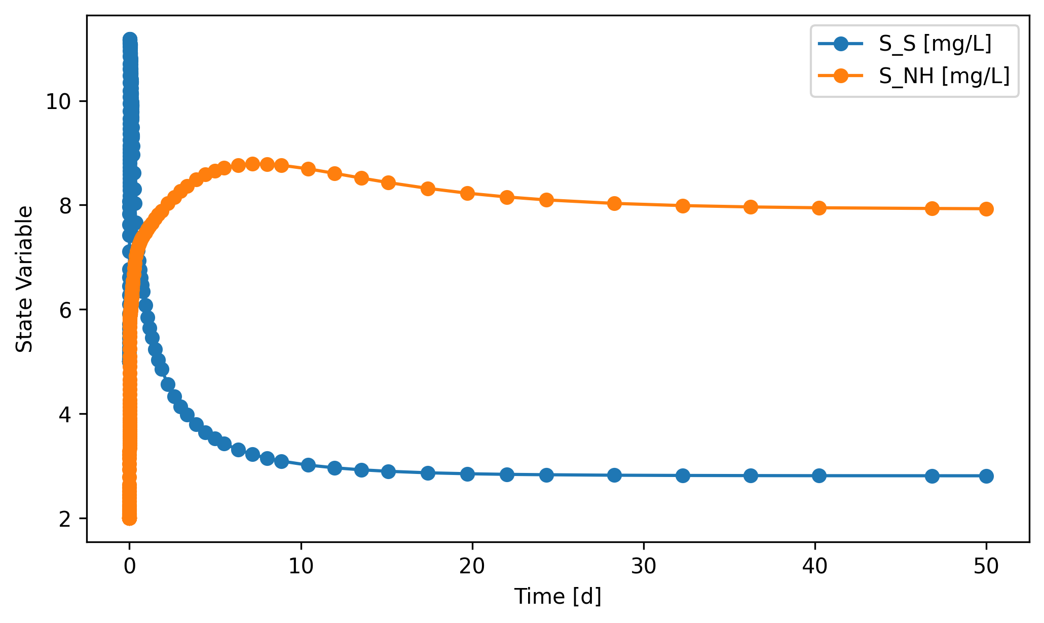
fig, ax = A1.scope.plot_time_series(('S_NH', 'S_S'))

Every SanUnit and WasteStream has a .scope attribute, but only the ones in sys.scope.subjects (shown above) actually accumulate data during a simulation. For everything else, the scope object exists but its record stays empty.

# Every SanUnit has a .scope attribute; here A2 is *not* in `sys.scope.subjects`
A2 = sys.flowsheet.unit.A2
A2.scope

<SanUnitScope: A2>

# ...but because A2 wasn't tracked, its record never got filled.
A2.scope.record

array([], shape=(0, 1), dtype=float64)

For A1, it is tracked, so each row in the record attribute is values of A1’s state variables at a certain time point.

# `time_series` stores the time data
A1.scope.time_series

array([0.000e+00, 5.098e-10, 1.020e-09, 6.117e-09, 1.122e-08, 6.219e-08,
       1.132e-07, 3.166e-07, 5.199e-07, 7.233e-07, 1.403e-06, 2.083e-06,
       2.763e-06, 8.673e-06, 1.458e-05, 2.049e-05, 3.168e-05, 4.287e-05,
       5.406e-05, 6.525e-05, 1.049e-04, 1.446e-04, 1.843e-04, 2.239e-04,
       3.091e-04, 3.942e-04, 4.793e-04, 5.645e-04, 6.496e-04, 8.359e-04,
       1.022e-03, 1.209e-03, 1.395e-03, 1.581e-03, 1.768e-03, 2.185e-03,
       2.602e-03, 2.896e-03, 3.189e-03, 3.399e-03, 3.567e-03, 3.736e-03,
       3.905e-03, 4.038e-03, 4.171e-03, 4.304e-03, 4.438e-03, 4.571e-03,
       4.704e-03, 4.849e-03, 4.993e-03, 5.138e-03, 5.283e-03, 5.427e-03,
       5.572e-03, 5.833e-03, 6.093e-03, 6.354e-03, 6.614e-03, 6.875e-03,
       7.332e-03, 7.790e-03, 8.248e-03, 8.706e-03, 9.409e-03, 1.011e-02,
       1.081e-02, 1.152e-02, 1.274e-02, 1.396e-02, 1.518e-02, 1.641e-02,
       1.848e-02, 2.055e-02, 2.195e-02, 2.335e-02, 2.426e-02, 2.516e-02,
       2.607e-02, 2.698e-02, 2.948e-02, 3.073e-02, 3.199e-02, 3.324e-02,
       3.386e-02, 3.449e-02, 3.511e-02, 3.730e-02, 3.949e-02, 4.168e-02,
       4.688e-02, 5.208e-02, 5.304e-02, 5.378e-02, 5.453e-02, 5.527e-02,
       5.601e-02, 5.719e-02, 5.836e-02, 5.954e-02, 6.201e-02, 6.447e-02,
       6.694e-02, 6.940e-02, 7.411e-02, 7.883e-02, 7.942e-02, 8.001e-02,
       8.060e-02, 8.126e-02, 8.193e-02, 8.259e-02, 8.325e-02, 8.392e-02,
       8.458e-02, 8.524e-02, 8.560e-02, 8.596e-02, 8.631e-02, 8.674e-02,
       8.717e-02, 8.763e-02, 8.809e-02, 9.040e-02, 9.270e-02, 9.500e-02,
       9.584e-02, 9.667e-02, 9.751e-02, 1.040e-01, 1.105e-01, 1.111e-01,
       1.116e-01, 1.122e-01, 1.175e-01, 1.229e-01, 1.239e-01, 1.248e-01,
       1.258e-01, 1.264e-01, 1.270e-01, 1.273e-01, 1.277e-01, 1.282e-01,
       1.286e-01, 1.292e-01, 1.298e-01, 1.304e-01, 1.333e-01, 1.362e-01,
       1.370e-01, 1.377e-01, 1.384e-01, 1.440e-01, 1.447e-01, 1.453e-01,
       1.471e-01, 1.488e-01, 1.606e-01, 1.724e-01, 1.738e-01, 1.753e-01,
       1.767e-01, 1.913e-01, 2.058e-01, 2.415e-01, 2.771e-01, 3.127e-01,
       3.741e-01, 4.356e-01, 4.970e-01, 5.584e-01, 6.171e-01, 6.757e-01,
       7.343e-01, 7.930e-01, 9.226e-01, 1.052e+00, 1.182e+00, 1.311e+00,
       1.498e+00, 1.684e+00, 1.871e+00, 2.241e+00, 2.612e+00, 2.983e+00,
       3.353e+00, 3.893e+00, 4.433e+00, 4.972e+00, 5.512e+00, 6.349e+00,
       7.186e+00, 8.023e+00, 8.860e+00, 1.042e+01, 1.198e+01, 1.354e+01,
       1.510e+01, 1.740e+01, 1.971e+01, 2.201e+01, 2.431e+01, 2.829e+01,
       3.227e+01, 3.625e+01, 4.022e+01, 4.682e+01, 5.000e+01])

The tracked time-series data can be exported to a file in two ways.

sys.scope.export('bsm1_time_series.xlsx')

or

import numpy as np
sys.simulate(state_reset_hook='reset_cache',
             t_span=(0, 50),
             t_eval=np.arange(0, 51, 1),
             method='BDF',
             export_state_to=('bsm1_time_series.xlsx'))

We can also (re-)define which unit or stream to track after the system has been constructed.

# Let's say we want to track the clarifier and the waste activated sludge
C1 = sys.flowsheet.unit.C1
WAS = sys.flowsheet.stream.WAS
sys.set_dynamic_tracker(C1, WAS)
sys.scope.subjects

(<FlatBottomCircularClarifier: C1>, <WasteStream: WAS>)

However, we would need to rerun the simulation to retrieve results.

# You can use a shorter time or try changing method to 'RK23' (explicit solver) if it takes a long time
sys.simulate(t_span=(0, 50), method='BDF', state_reset_hook='reset_cache')
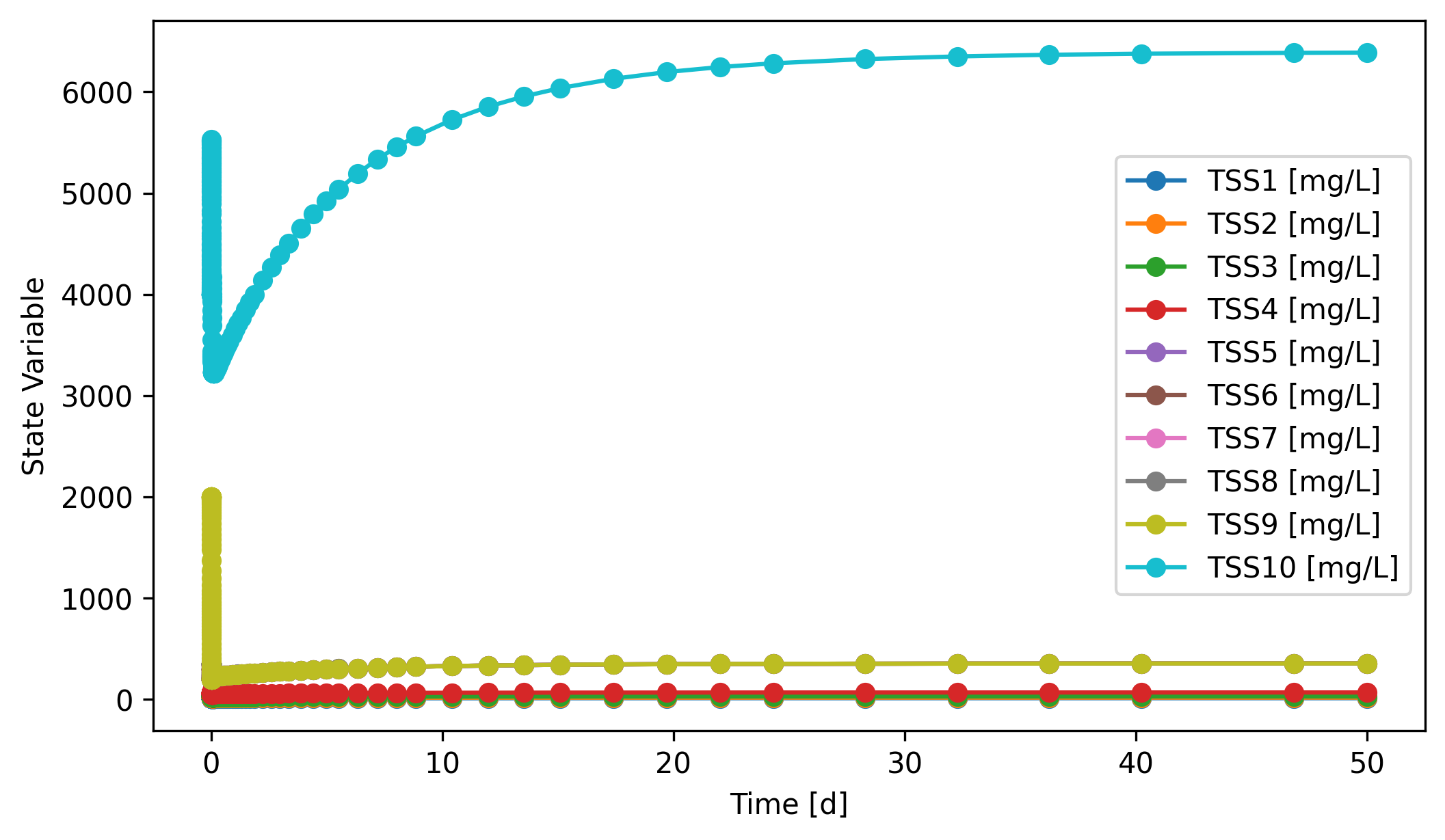
# The clarifier are modeled as 10 layers, so we can track the TSS in each layer
fig, ax = C1.scope.plot_time_series([f'TSS{i}' for i in range(1,11)])

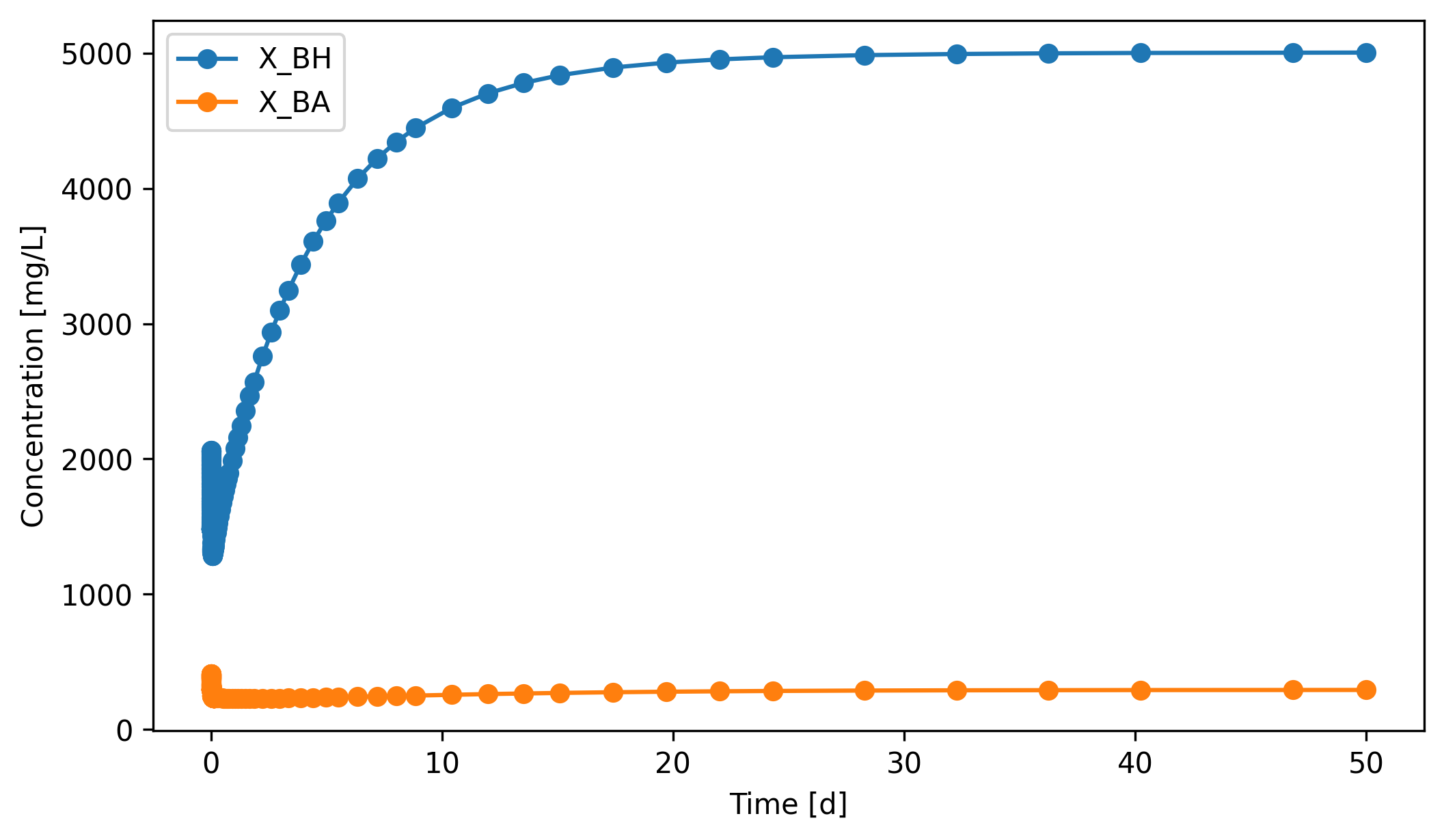
fig, ax = WAS.scope.plot_time_series(('X_BH', 'X_BA'))

So far we’ve learned how to simulate any dynamic system developed with QSDsan. A complete list of existing unit operations within QSDsan is available in the documentation. Unit operations labeled as “QSDsan dynamic” are enabled for dynamic simulations. Any system composed of the enabled units can be simulated dynamically as we learned above.

1.2. When is a system “dynamic”?

It’s ultimately the user’s decision whether a system should be run dynamically. This section will cover the essentials to switch to the dynamic mode for system simulation.

1.2.1. System.isdynamic vs. SanUnit.isdynamic vs. SanUnit.hasode

• Simply speaking, when <System>.isdynamic is True, the program will attempt dynamic simulation. Users can directly enable/disable the dynamic mode by setting the isdynamic property of a System object.

• The program will set the value of <System>.isdynamic when it’s not specified by users. <System>.isdynamic is considered True in all cases except when <SanUnit>.isdynamic is False for all units.

• Setting <SanUnit>.isdynamic = True does not guarantee the unit can be simulated dynamically. Just like how the _run method must be defined for static simulation, a series of additional methods must be defined to enable dynamic simulation.

• If a unit operation has ODE algorithms, i.e., <SanUnit>.hasode is True, it means a unit has the fundamental methods to compile ODEs. This is a sufficient but not necessary condition for dynamic simulation, because a unit doesn’t have to be described with ODEs to be capable of dynamic simulations.

# All units in the BSM1 system above have ODEs
{u: u.hasode for u in sys.units}

{<CSTR: A1>: True,
 <CSTR: A2>: True,
 <CSTR: O1>: True,
 <CSTR: O2>: True,
 <CSTR: O3>: True,
 <FlatBottomCircularClarifier: C1>: True}

2. Writing a dynamic SanUnit

Whether a system can be simulated dynamically ultimately boils down to whether all the units in the system have the fundamental methods required for dynamic simulations. In this section, you’ll learn how to implement your own algorithms to create a SanUnit subclass capable of dynamic simulations.

2.1. How the integrator drives a dynamic unit

Before getting into the per-method mechanics in §2.2 and §2.3, it helps to picture how the integrator orchestrates a dynamic system over one step. The figure below shows one update cycle.

Per step: solve_ivp passes (t, y) down. Each unit’s _compile_AE / _compile_ODE writes its _state and _dstate. _update_state / _update_dstate write the unit’s state into each outlet WasteStream. The downstream unit reads its inlets’ .state / .dstate as y_ins / dy_ins. The aggregated dy/dt (across the system’s ODE state) is returned to solve_ivp, which advances time.

A few things to note from this picture:

• State lives in two places. Each SanUnit keeps its own _state / _dstate arrays (what the unit’s algorithm is computing); each WasteStream keeps its state / dstate arrays (the inlets the next unit reads). The two are not the same buffer. _update_state and _update_dstate are the bridge: they’re called inside the unit’s compiled function so the outlet stream sees the latest values.

• Units communicate only through streams. A downstream unit never reads its upstream’s _state directly — it reads its inlets’ state (and dstate) as y_ins (and dy_ins).

• One global state vector. The integrator’s y vector is the concatenation of the ODE-state of every unit. solve_ivp doesn’t know about streams; it just sees one big state vector.

2.1.1. _compile_AE vs. _compile_ODE: which one when?

_compile_AE (for algebraic equation units) and _compile_ODE (for ordinary differential equation units) both fit the same data-flow diagram, but they describe different physics.

• _compile_ODE — use when the unit has holdup or inertia: tanks, reactors, settlers, anywhere a balance reads d(state)/dt = inflow − outflow + reactions. The function you compile populates _dstate; the integrator integrates it.

• _compile_AE — use when the unit’s state is instantaneously determined by its inputs: mixers, splitters, pumps without holdup, hydraulic delays. There is no time derivative to integrate; the function you compile sets _state directly each time the integrator asks for the system’s state.

Mixed systems work naturally: AE units act as pass-throughs within each integrator step, while ODE units are what solve_ivp actually integrates. If you find yourself writing dy_dt = 0 for everything in a unit, you probably wanted _compile_AE instead.

Tip: A unit declares its choice by implementing the corresponding _compile_* method and exposing the matching AE or ODE property (you’ll see both patterns in §2.4 and §2.5). A unit can implement only one of the two: an ODE unit doesn’t need an AE; an AE unit doesn’t need an ODE.

2.2. Basic structure

During static system simulations, _run directly defines the mass and/or energy flows of the effluent WasteStream objects of the unit after calculation.

In comparison, during dynamic simulations, all information are stored as _state and _dstate attributes of the relevant SanUnit objects as well as state and dstate properties of WasteStream objects. These information won’t be translated to mass or energy flows until dynamic simulation is completed.

• WasteStream.state is a 1d numpy.array of length \(n+1\), \(n\) is the length of the components associated with the thermo. Each element of the array represents value of one state variable.

Tip: When the dynamic simulation finishes, QSDsan reconstructs each WasteStream’s mass flow as state[:-1] * state[-1] (in g/d). That product determines what the two conventions below mean.

• Liquid ``WasteStream`` (the default): the first \(n\) elements are component concentrations [mg/L = g/m³] and the last element is the total volumetric flow [m³/d]. Their product gives mass flow [g/d].

• Gaseous ``WasteStream``: a gas’s volumetric flow at the operating \(T\) and \(P\) depends on composition, so working in concentrations is awkward. As the same state[:-1] * state[-1] algorithm still has to produce mass flow, so the convention is to store the component mass flows [g/d] directly in the first \(n\) elements and fix the last element at \(1\), so the reconstructed mass flow is whatever you stored.

• WasteStream.dstate is an array of the exact same shape as WasteStream.state, storing values of the time derivatives (i.e., the rates of change) of the state variables.

sf = sys.flowsheet.stream
sf.effluent.dstate.shape == sf.effluent.state.shape

True

SanUnit._state is also a 1d numpy.array, but the length of the array is not assumed, because the state variables relevant for a SanUnit is entirely dependent on the unit operation itself. Therefore, there is no predefined units of measure or order for state variables of a unit operation.

C1._state.shape == A1._state.shape
# C1._state.shape == C1._dstate.shape

False

But similar to WasteStream, SanUnit._dstate must have the exact same shape as the _state array, as each element corresponds to the time derivative of a state variable.

# Some dynamic units in QSDsan have a `state` property that formats
# the data in `_state` for better readability
A1.state

{'S_I': 30.0,
 'S_S': 2.8098492768502354,
 'X_I': 1147.9023456598527,
 'X_S': 82.1496729433189,
 'X_BH': 2551.149645860236,
 'X_BA': 148.1855399395735,
 'X_P': 447.1138645933302,
 'S_O': 0.004288922586191978,
 'S_NO': 5.338947439089076,
 'S_NH': 7.9289428538204,
 'S_ND': 1.216685860427014,
 'X_ND': 5.285736721431849,
 'S_ALK': 59.15831466857708,
 'S_N2': 25.00787300530831,
 'H2O': 997375.2641947934,
 'Q': 92230.0}

2.3. Fundamental methods

In addition to proper __init__ and _run methods (SanUnit advanced tutorial), a few more methods are required in a SanUnit subclass for dynamic simulation. Users typically won’t interact with these methods but they will be called by System.simulate to manipulate the values of the arrays mentioned above (i.e., <SanUnit>._state, <SanUnit>._dstate, <WasteStream>.state, and <WasteStream>.dstate).

• _init_state, called after _run to generate an initial condition for the unit, i.e., defining shape and values of the _state and _dstate arrays. For example:

import numpy as np
def _init_state(self):
    inf = self.ins[0]
    self._state = np.ones(len(inf.components)+1)
    self._dstate = self._state * 0.

This method (not saying it makes sense) assumes \(n+1\) state variables and gives an initial value of 1 to all of them. Then it also sets the initial time derivatives to be 0.

• _update_state, to update effluent streams’ state arrays based on current state (and maybe dstate) of the SanUnit. For example:

def _update_state(self):
    arr = self._state   # retrieving the current state of the SanUnit
    eff, = self.outs    # assuming this SanUnit has one outlet only
    eff.state[:] = arr  # assume arr has the same shape as WasteStream.state

The goal of this method is to update the values in <WasteStream>.state for each WasteStream in <SanUnit>.outs.

• _update_dstate, to update effluent streams’ dstate arrays based on current _state and _dstate of the SanUnit. The signature and often the algorithm are similar to _update_state.

• _compile_ODE or _compile_AE, used to define the function that updates the _dstate and/or _state of the SanUnit based on its influent streams’ state/dstate and potentially its own current state. The defined function will be stored as SanUnit._ODE or SanUnit._AE. These methods should follow some general forms like below:

@property
def ODE(self):
    if self._ODE is None:
        self._compile_ODE()
    return self._ODE

def _compile_ODE(self):
    _dstate = self._dstate
    _update_dstate = self._update_dstate
    def dy_dt(t, y_ins, y, dy_ins):
        _dstate[:] = some_algorithm(t, y_ins, y, dy_ins)
        _update_dstate()
    self._ODE = dy_dt

@property
def AE(self):
    if self._AE is None:
        self._compile_AE()
    return self._AE

def _compile_AE(self):
    _state = self._state
    _dstate = self._dstate
    _update_state = self._update_state
    _update_dstate = self._update_dstate
    def y_t(t, y_ins, dy_ins):
        _state[:] = some_algorithm(t, y_ins, dy_ins)
        _dstate[:] = some_other_algorithm(t, y_ins, dy_ins)
        _update_state()
        _update_dstate()
    self._AE = y_t

Note: When writing the dy_dt or y_t functions, use <SanUnit>._state[:] = <new_value> rather than <SanUnit>._state = <new_value> because it’s generally faster to update values in an existing array than overwriting this array with a newly created array.

In the next subsection, we’ll learn more about the ODE and AE methods.

2.4. Making a simple MixerSplitter (_compile_AE)

Let’s say we want to make an ideal mixer-splitter that instantly mixes all streams at the inlets and then evenly split them across the outlets.

# Typically if implemented as a static SanUnit, it'd be pretty simple
# Let's ignore `_design` and `_cost` for now.
class MixerSplitter1(qs.SanUnit):
    _N_outs = 3
    _ins_size_is_fixed = False
    _outs_size_is_fixed = False
    def __init__(self, ID='', ins=None, outs=(), thermo=None,
                 init_with='WasteStream', **kwargs):
        qs.SanUnit.__init__(self, ID, ins, outs, thermo, init_with, **kwargs)
        self.mixed = qs.WasteStream()

    def _run(self):
        mixed = self.mixed
        mixed.mix_from(self.ins)
        n_outs = len(self.outs)
        flow = mixed.get_total_flow('kg/hr')/n_outs
        for out in self.outs:
            out.copy_like(mixed)
            out.set_total_flow(flow, 'kg/hr')

    def _design(self):
        pass

    def _cost(self):
        pass

# Let's try simulating it with the components used in BSM1
cmps = qs.get_thermo().chemicals
cmps.show()

CompiledComponents([
    S_I,   S_S,  X_I,  X_S,
    X_BH,  X_BA, X_P,  S_O,
    S_NO,  S_NH, S_ND, X_ND,
    S_ALK, S_N2, H2O,
])

# Now let's make a couple fake influents
inf1 = qs.WasteStream('inf1', H2O=1000, S_O=5)
inf2 = qs.WasteStream('inf2', H2O=800, S_S=3, S_NH=2.1)
inf2.show()

WasteStream: inf2
phase: 'l', T: 298.15 K, P: 101325 Pa
flow (g/hr): S_S   3e+03
             S_NH  2.1e+03
             H2O   8e+05
 WasteStream-specific properties:
  pH         : 7.0
  Alkalinity : 2.5 mmol/L
  COD        : 3708.6 mg/L
  BOD        : 2659.0 mg/L
  TC         : 1186.7 mg/L
  TOC        : 1186.7 mg/L
  TN         : 2596.0 mg/L
  TP         : 37.1 mg/L
 Component concentrations (mg/L):
  S_S    3708.6
  S_NH   2596.0
  H2O    988949.8

MS1 = MixerSplitter1(ins=(inf1, inf2))
MS1.simulate()
MS1.show()

MixerSplitter1: M1
ins...
[0] inf1
phase: 'l', T: 298.15 K, P: 101325 Pa
flow (g/hr): S_O  5e+03
                H2O  1e+06
    WasteStream-specific properties:
     pH         : 7.0
     Alkalinity : 2.5 mmol/L
[1] inf2
phase: 'l', T: 298.15 K, P: 101325 Pa
flow (g/hr): S_S   3e+03
                S_NH  2.1e+03
                H2O   8e+05
    WasteStream-specific properties:
     pH         : 7.0
     Alkalinity : 2.5 mmol/L
     COD        : 3708.6 mg/L
     BOD        : 2659.0 mg/L
     TC         : 1186.7 mg/L
     TOC        : 1186.7 mg/L
     TN         : 2596.0 mg/L
     TP         : 37.1 mg/L
outs...
[0] ws11
phase: 'l', T: 298.15 K, P: 101325 Pa
flow (g/hr): S_S   1e+03
                S_O   1.67e+03
                S_NH  700
                H2O   6e+05
    WasteStream-specific properties:
     pH         : 7.0
     Alkalinity : 2.5 mmol/L
     COD        : 1650.2 mg/L
     BOD        : 1183.2 mg/L
     TC         : 528.1 mg/L
     TOC        : 528.1 mg/L
     TN         : 1155.1 mg/L
     TP         : 16.5 mg/L
[1] ws12
phase: 'l', T: 298.15 K, P: 101325 Pa
flow (g/hr): S_S   1e+03
                S_O   1.67e+03
                S_NH  700
                H2O   6e+05
    WasteStream-specific properties:
     pH         : 7.0
     Alkalinity : 2.5 mmol/L
     COD        : 1650.2 mg/L
     BOD        : 1183.2 mg/L
     TC         : 528.1 mg/L
     TOC        : 528.1 mg/L
     TN         : 1155.1 mg/L
     TP         : 16.5 mg/L
[2] ws13
phase: 'l', T: 298.15 K, P: 101325 Pa
flow (g/hr): S_S   1e+03
                S_O   1.67e+03
                S_NH  700
                H2O   6e+05
    WasteStream-specific properties:
     pH         : 7.0
     Alkalinity : 2.5 mmol/L
     COD        : 1650.2 mg/L
     BOD        : 1183.2 mg/L
     TC         : 528.1 mg/L
     TOC        : 528.1 mg/L
     TN         : 1155.1 mg/L
     TP         : 16.5 mg/L

# Obviously, it's not ready for dynamic simulation
# You will receive an error if you try to simulate it with `isdynamic=True`
MS1_dyn = MixerSplitter1(ins=(inf1.copy(), inf2.copy()), isdynamic=True)
dyn_sys = qs.System(path=(MS1_dyn,))
dyn_sys.simulate(t_span=(0,5))

---------------------------------------------------------------------------
AttributeError                            Traceback (most recent call last)
Cell In[26], line 5
      1 # Obviously, it's not ready for dynamic simulation
      2 # You will receive an error if you try to simulate it with `isdynamic=True`
      3 MS1_dyn = MixerSplitter1(ins=(inf1.copy(), inf2.copy()), isdynamic=True)
      4 dyn_sys = qs.System(path=(MS1_dyn,))
----> 5 dyn_sys.simulate(t_span=(0,5))

File ~\Documents\Coding\QSDsan-platform\.venv\Lib\site-packages\biosteam\_system.py:3374, in System.simulate(self, update_configuration, units, design_and_cost, **kwargs)
   3354 def simulate(self, update_configuration: Optional[bool]=None, units=None,
   3355              design_and_cost=None, **kwargs):
   3356     """
   3357     If system is dynamic, run the system dynamically. Otherwise, converge 
   3358     the path of unit operations to steady state. After running/converging 
   (...)   3372         
   3373     """
-> 3374     with self.flowsheet:
   3375         specifications = self._specifications
   3376         if specifications and not self._running_specifications:

File ~\Documents\Coding\QSDsan-platform\.venv\Lib\site-packages\biosteam\_flowsheet.py:120, in Flowsheet.__exit__(self, type, exception, traceback)
    118 def __exit__(self, type, exception, traceback):
    119     main_flowsheet.set_flowsheet(self._temporary_stack.pop())
--> 120     if exception: raise exception

File ~\Documents\Coding\QSDsan-platform\.venv\Lib\site-packages\biosteam\_system.py:3418, in System.simulate(self, update_configuration, units, design_and_cost, **kwargs)
   3416 self._setup(update_configuration, units)
   3417 if self.isdynamic:
-> 3418     outputs = self.dynamic_run(**kwargs)
   3419     if design_and_cost: self._summary()
   3420 else:

File ~\Documents\Coding\QSDsan-platform\.venv\Lib\site-packages\biosteam\_system.py:3509, in System.dynamic_run(self, **dynsim_kwargs)
   3507 # Load initial states
   3508 self.converge()
-> 3509 y0, idx, nr = self._load_state()
   3510 dk['y0'] = y0
   3511 # Integrate

File ~\Documents\Coding\QSDsan-platform\.venv\Lib\site-packages\biosteam\_system.py:3206, in System._load_state(self)
   3204 idx = {}
   3205 for unit in units:
-> 3206     unit._init_state()
   3207     unit._update_state()
   3208     unit._update_dstate()

AttributeError: 'MixerSplitter1' object has no attribute '_init_state'

Since the mixer-splitter mixes and splits instantly, we can express this process with a set of algebraic equations (AEs). Assume its array of state variables follow the “concentration-volumetric flow” convention. In mathematical forms, state variables of the mixer-splitter (\(C_m\), component concentrations; \(Q_m\), total volumetric flow) follow:

\[Q_m = \sum_{i \in ins} Q_i \tag{1}\]

\[Q_mC_m = \sum_{i \in ins} Q_iC_i\]

\[\therefore C_m = \frac{\sum_{i \in ins} Q_iC_i}{Q_m} \tag{2}\]

Therefore, the time derivatives \(\dot{Q_m}\) follow:

\[\dot{Q_m} = \sum_{i \in ins} \dot{Q_i} \tag{3}\]

\[Q_m\dot{C_m} + C_m\dot{Q_m} = \sum_{i \in ins} (Q_i\dot{C_i} + C_i\dot{Q_i})\]

\[\therefore \dot{C_m} = \frac{1}{Q_m}\cdot(\sum_{i \in ins}Q_i\dot{C_i} + \sum_{i \in ins}C_i\dot{Q_i} - C_m\dot{Q_m}) \tag{4}\]

For any effluent WasteStream \(j\):

\[Q_j = \frac{Q_m}{n_{outs}} \tag{5}\]

\[C_j = C_m \tag{6}\]

\[\therefore \dot{Q_j} = \frac{\dot{Q_m}}{n_{outs}} \tag{7}\]

\[\dot{C_j} = \dot{C_m} \tag{8}\]

The diagram below uses an illustrative case with \(m = 3\) inlets and \(n = 4\) components; the same shapes generalize to any m and n. Equation (1) is Q_m = sum(Q_ins), equation (2) is the flow-weighted concentration C_m = Q_ins · C_ins / Q_m, and equations (5)–(8) just slice the result across the outlets.

The matrix product Q_ins · C_ins yields an n-vector of flow-weighted sums, which divided by Q_m gives the mixer’s component concentrations.

Now, let’s try to implement this algorithm in methods for dynamic simulation.

import numpy as np
class MixerSplitter2(MixerSplitter1):
    def _init_state(self):
        mixed = self.mixed
        self._state = np.empty(len(cmps)+1)
        self._state[:-1] = mixed.conc  # first n element be the component concentrations of the mixed stream
        self._state[-1] = mixed.F_vol * 24 # last element be the total volumetric flow, in m3/d
        self._dstate = self._state * 0.

    def _update_state(self):
        y = self._state
        n_outs = len(self.outs)
        for ws in self.outs:
            if ws.state is None: ws.state = y.copy() # initialize the state using a copy
            else: ws.state[:-1] = y[:-1] # equation (6)
            ws.state[-1] = y[-1]/n_outs  # equation (5)

    def _update_dstate(self):
        dy = self._dstate
        n_outs = len(self.outs)
        for ws in self.outs:
            if ws.dstate is None: ws.dstate = dy.copy()
            else: ws.dstate[:-1] = dy[:-1]  # equation (8)
            ws.dstate[-1] = dy[-1]/n_outs   # equation (7)

    @property
    def AE(self):
        if self._AE is None:
            self._compile_AE()
        return self._AE

    def _compile_AE(self):
        _state = self._state
        _dstate = self._dstate
        _update_state = self._update_state
        _update_dstate = self._update_dstate
        def y_t(t, y_ins, dy_ins):
            Q_ins = y_ins[:,-1]
            C_ins = y_ins[:,:-1]
            dQ_ins = dy_ins[:,-1]
            dC_ins = dy_ins[:,:-1]
            _state[-1] = Q = sum(Q_ins)           # equation (1)
            _state[:-1] = C = Q_ins @ C_ins / Q   # equation (2)
            _dstate[-1] = dQ = sum(dQ_ins)        # equation (3)
            _dstate[:-1] = dC = (Q_ins @ dC_ins + dQ_ins @ C_ins - C*dQ) / Q  # equation (4)
            _update_state()
            _update_dstate()
        self._AE = y_t

Note: 1. All SanUnit._AE must take exactly these three positional arguments (t, y_ins, dy_ins). t is time as a float. Both y_ins and dy_ins are 2d numpy.array of the same shape (m, n+1), where \(m\) is the number of inlets, \(n+1\) is the length of the state or dstate array of a WasteStream.

2. All SanUnit._AE must update both _state and _dstate of the SanUnit, and must call _update_state and _update_dstate afterwards.

# Now let's see if this works
MS2 = MixerSplitter2(ins=(inf1.copy(), inf2.copy()), isdynamic=True)
dyn_sys2 = qs.System(path=(MS2,))
dyn_sys2.set_dynamic_tracker(MS2)
dyn_sys2.simulate(t_span=(0,5))

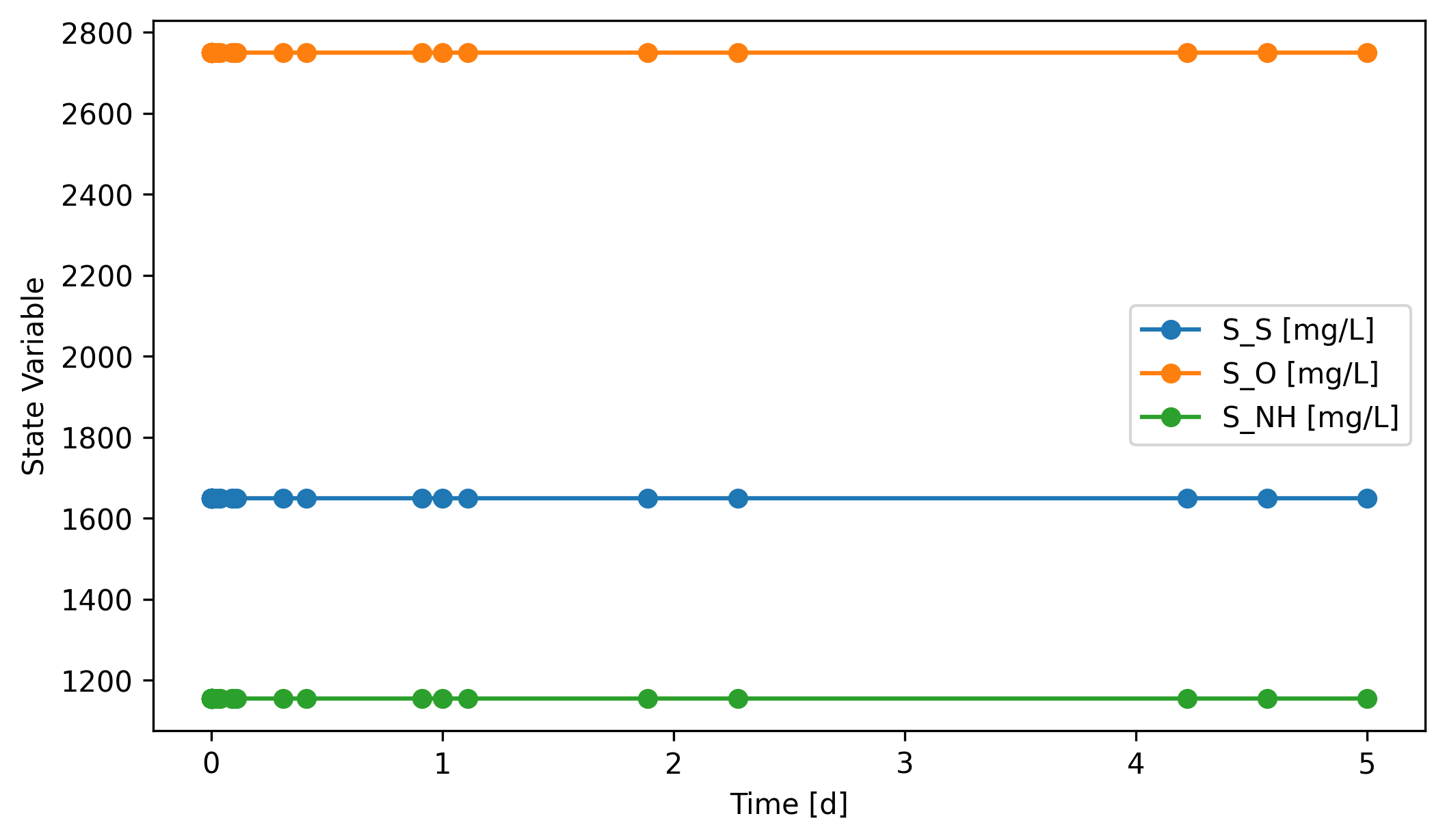
# You'll see the mass flows stay constant through the simulation period,
# but still it means the system was simulated dynamically.
fig, ax = MS2.scope.plot_time_series(('S_S', 'S_NH', 'S_O'))

Many commonly used unit operations, such as Pump, Mixer, Splitter, and HydraulicDelay, have implemented the fundamental methods to be used in a dynamic system. You can always refer to the source codes of these units to learn more about how they work.

2.5. Making an inactive CompleteMixTank (_compile_ODE)

As you can see above, it’s not very useful to dynamically simulate a system without any ODEs. So let’s make a simple inactive complete mix tank (inactive means no reactions). Assume the reactor has a fixed liquid volume \(V\), and thus the effluent volumetric flow rate changes instantly with influents. The mass balance of this type of reactor can be described as:

\[Q = \sum_{i \in ins} Q_i \tag{9}\]

\[\therefore \dot{Q} = \sum_{i \in ins} \dot{Q_i} \tag{10}\]

\[\frac{d(VC)}{dt} = \sum_{i \in ins} Q_iC_i - QC\]

\[\therefore \dot{C} = \frac{1}{V}(\sum_{i \in ins} Q_iC_i - QC) \tag{11}\]

Equations (10) and (11) are the governing ODEs of this unit.

A fixed-volume CSTR with instant mixing. The unit’s state is what’s in the tank: an n-vector of concentrations C and a scalar volumetric flow Q. The integrator advances both via the ODE shown.

Notice the asymmetry with the MixerSplitter: there, state was algebraically determined by the inlets at each step. Here, state has inertia (the holdup V), so it needs a real dy/dt.

class CompleteMixTank(qs.SanUnit):

    _N_outs = 1
    _ins_size_is_fixed = False

    def __init__(self, ID='', ins=None, outs=(), thermo=None,
                 init_with='WasteStream', V=10, **kwargs):
        qs.SanUnit.__init__(self, ID, ins, outs, thermo, init_with, **kwargs)
        self.V = V

    def _run(self):
        out, = self.outs
        out.mix_from(self.ins)

    def set_init_conc(self,**concentrations):
        cmps = self.thermo.chemicals
        C = np.zeros(len(cmps))
        idx = cmps.indices(list(concentrations.keys()))
        C[idx] = list(concentrations.values())
        self._init_concs = C

    def _init_state(self):
        out, = self.outs
        self._state = np.empty(len(cmps)+1)
        self._state[:-1] = self._init_concs      # first n element be the component concentrations of the mixed stream
        self._state[-1] = out.F_vol*24   # last element be the total volumetric flow
        self._dstate = self._state*0.

    def _update_state(self):
        out, = self.outs
        out.state = self._state

    def _update_dstate(self):
        out, = self.outs
        out.dstate = self._dstate

    @property
    def ODE(self):
        if self._ODE is None:
            self._compile_ODE()
        return self._ODE

    def _compile_ODE(self):
        _dstate = self._dstate
        _update_dstate = self._update_dstate
        V = self.V
        def dy_dt(t, y_ins, y, dy_ins):
            Q_ins = y_ins[:,-1]
            C_ins = y_ins[:,:-1]
            dQ_ins = dy_ins[:,-1]
            Q = sum(Q_ins)   # equation (9)
            C = y[:-1]
            _dstate[-1] = sum(dQ_ins) # dQ, equation (10)
            _dstate[:-1] = (Q_ins @ C_ins - Q*C)/V # dC, equation (11)
            _update_dstate()
        self._ODE = dy_dt

Note: 1. All SanUnit._ODE must take exactly these four positional arguments: t, y_ins, and dy_ins are the same as the ones in SanUnit._AE. y is a 1d numpy.array, because it is equal to the _state array of the unit.

2. Unlike _AE, all SanUnit._ODE updates only the _dstate array of the SanUnit, and only calls _update_dstate afterwards.

# Let's see if it works
CMT = CompleteMixTank(ins=(inf1.copy(), inf2.copy()), V=50,
                      isdynamic=True)
dyn_sys3 = qs.System(path=(CMT,))
dyn_sys3.set_dynamic_tracker(CMT)

# We set the initial condition to be different from the steady state,
# so we can see how the system evolves to the steady state.
CMT.set_init_conc(S_S=500, S_NH=700, S_O=290)
dyn_sys3.simulate(t_span=(0,5))

CMT.scope.plot_time_series(('S_NH', 'S_S', 'S_O'))

(<Figure size 2400x1350 with 1 Axes>,
 <Axes: xlabel='Time [d]', ylabel='State Variable'>)

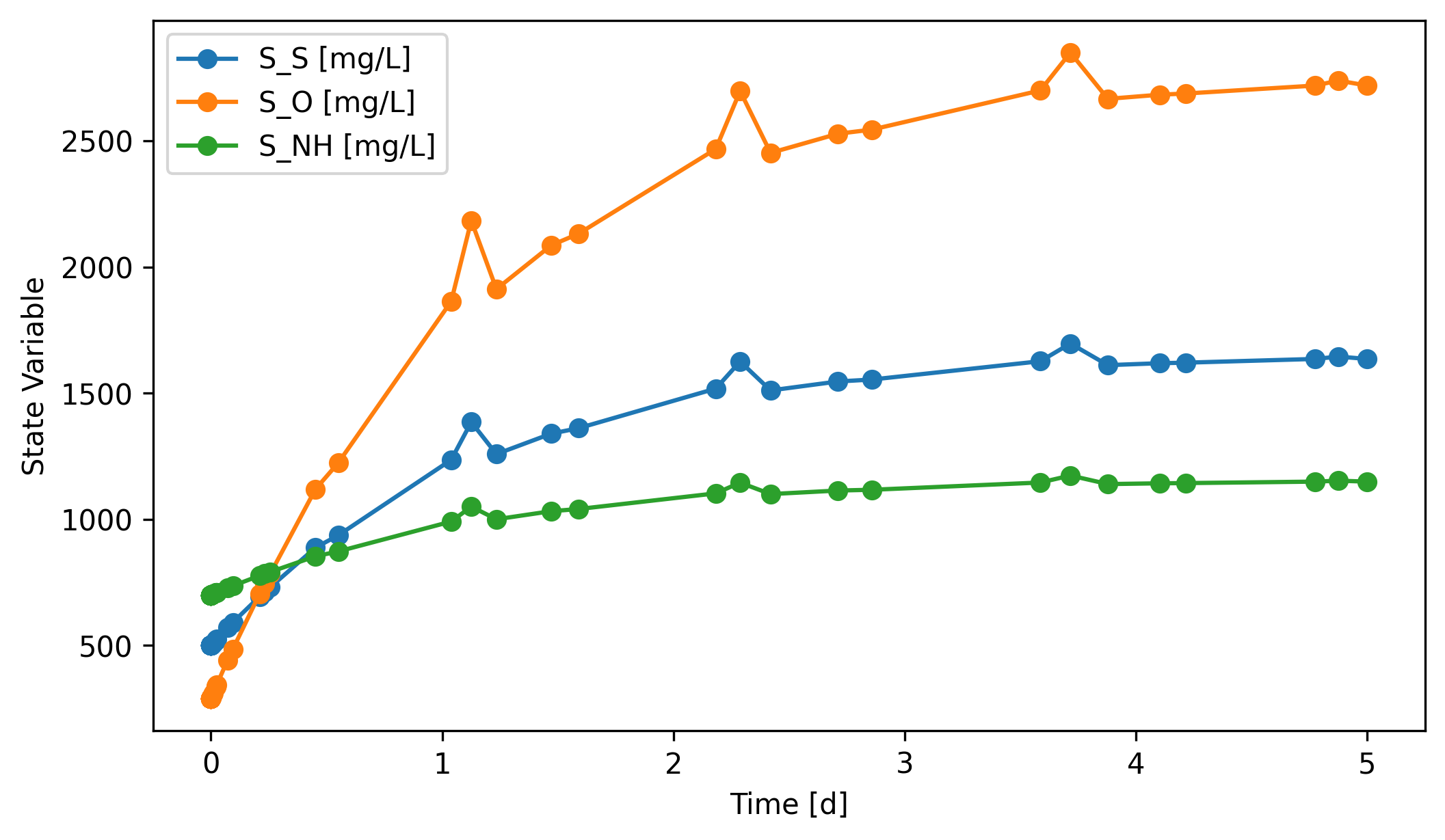
Many commonly used unit operations described by ODEs have been implemented in QSDsan, such as CSTR, BatchExperiment, and FlatBottomCircularClarifier.

3. Other convenient features

3.1. ExogenousDynamicVariable

The ExogenousDynamicVariable class is created to enable incorporation of exogenous dynamic variables in unit simulations. By “dynamic”, it means the variable value changes over time. By “exogenous”, it means the variable isn’t explicitly dependent on any unit operation or stream. “Ambient temperature” or “sunlight irradiance” is a good example. They are environmental conditions that are often beyond control but have an effect on the operation or performance of the system.

There are generally two ways to create an ExogenousDynamicVariable:

1. Define the variable as a function of time. Let’s say we want to create a variable to represent the changing reaction temperature. Assume the temperature value [K] can be expressed as \(T = 298.15 + 5\cdot \sin(t)\), indicating that the temperature fluctuates around \(25^{\circ}C\) by \(\pm 5^{\circ}C\). Then simply,

T = EDV('T', function=lambda t: 298.15+5*np.sin(t))

2. Provide time-series data to describe the dynamics of the variable. For demonstration purpose, we’ll just make up the data. In practice, this should be used if you have real data (e.g., knowing the change of temperature over time).

t_arr = np.linspace(0, 5)
y_arr = 298.15+5*np.sin(t_arr)
T = EDV('T', t=t_arr, y=y_arr)

Once created, these ExogenousDynamicVariable objects can be incorporated into any SanUnit upon its initialization or through the SanUnit.exo_dynamic_vars property setter.

# Let's see an example
from exposan.metab import create_system
sys_mt = create_system()
uf_mt = sys_mt.flowsheet.unit
uf_mt.R1.exo_dynamic_vars

All impact items have been removed from the registry.

C:\Users\Yalin\Documents\Coding\QSDsan-platform\.venv\Lib\site-packages\thermosteam\_stream.py:407: RuntimeWarning: <Stream: _mixed> has been replaced in registry
  self._register(ID)

(<ExogenousDynamicVariable: T>,)

# The evaluation of these variables during unit simulation is done through
# the `eval_exo_dynamic_vars` method
uf_mt.R1.eval_exo_dynamic_vars(t=0.1)

[295.15]

3.1.1. Batch construction from a file

EDV.batch_init is the easiest way to define several variables at once. It expects a CSV/Excel file with a t column and one extra column per variable.

from qsdsan.utils import ExogenousDynamicVariable as EDV
import os, tempfile
import pandas as pd

# Build a small time series in memory; in practice this would be a logged
# data file (e.g., ambient temperature and sunlight irradiance).
tmpdir = tempfile.mkdtemp()
csv_path = os.path.join(tmpdir, 'env_vars.csv')
t = np.linspace(0, 5, 51)
pd.DataFrame({
    't': t,
    'T': 293.15 + 5.0 * np.sin(2 * np.pi * t / 2.0),   # 20 +/- 5 degC, 2-day period
    'I': 400.0 + 200.0 * np.sin(2 * np.pi * t / 1.0),  # made-up irradiance, 1-day period
}).to_csv(csv_path, index=False)

# `batch_init` returns one `ExogenousDynamicVariable` per non-`t` column.
edvs = EDV.batch_init(csv_path)
edvs

[<ExogenousDynamicVariable: T>, <ExogenousDynamicVariable: I>]

3.1.2. Using an EDV inside a custom dynamic SanUnit

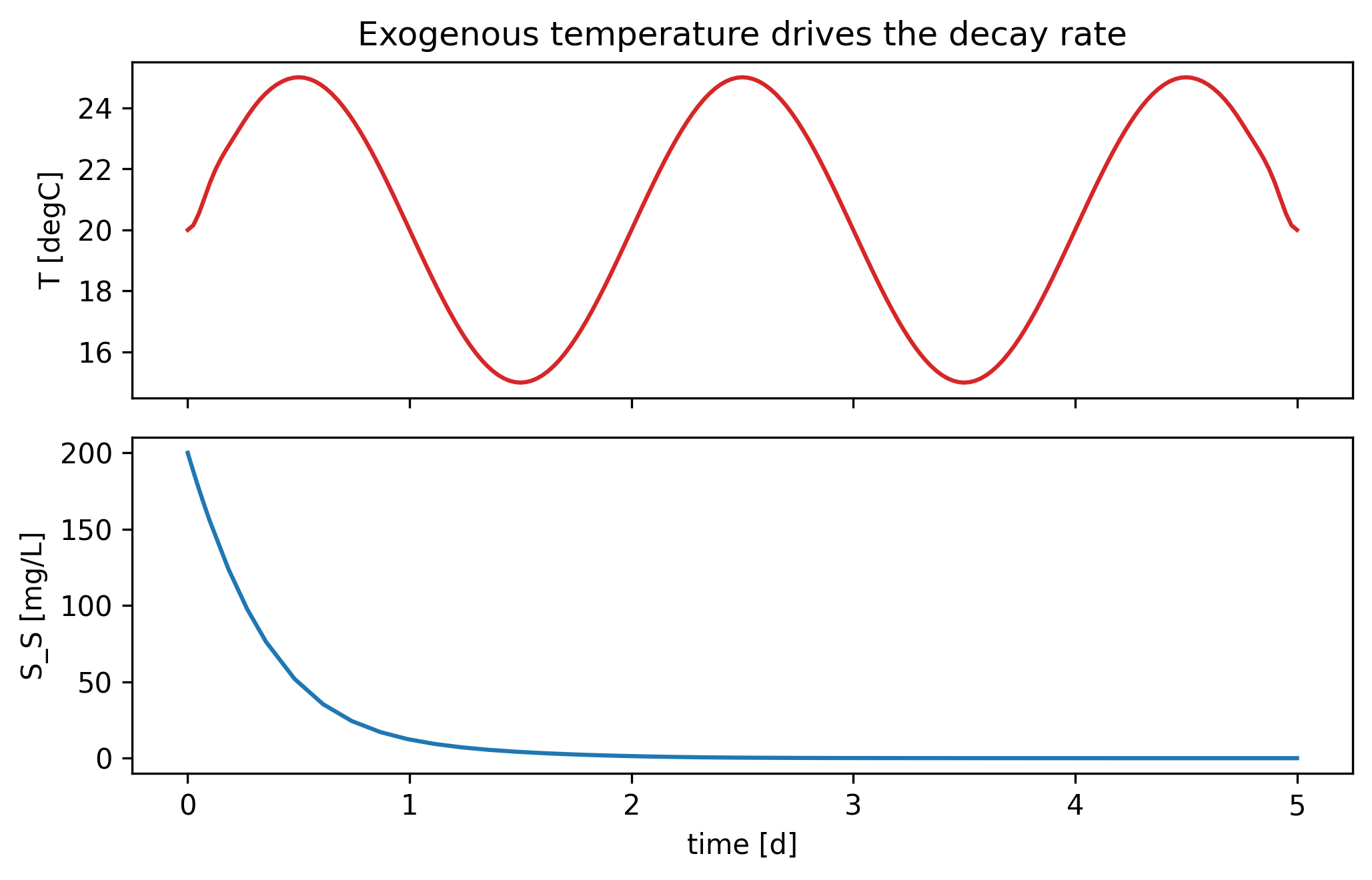
To plug an EDV into a SanUnit, pass it (or several) via exogenous_vars= at construction. Inside _compile_ODE or _compile_AE, call self.eval_exo_dynamic_vars(t) to read the current values. The example below extends the CompleteMixTank from §2.5 with a temperature-dependent first-order decay rate on one chosen component, using an Arrhenius form \(k(T) = k_{ref}\, \exp\!\left(\frac{E_a}{R}\left(\frac{1}{T_{ref}} - \frac{1}{T}\right)\right)\).

class EnvAwareCMT(CompleteMixTank):
    """CompleteMixTank with a temperature-dependent first-order decay on one component."""
    def __init__(self, ID='', ins=None, outs=(), V=10, target='S_S',
                 k_ref=2.0, T_ref=293.15, Ea_R=4000.0,
                 exogenous_vars=(), **kwargs):
        super().__init__(ID=ID, ins=ins, outs=outs, V=V,
                         exogenous_vars=exogenous_vars, **kwargs)
        self._idx = self.thermo.chemicals.index(target)
        self.k_ref, self.T_ref, self.Ea_R = k_ref, T_ref, Ea_R

    @property
    def ODE(self):
        if self._ODE is None: self._compile_ODE()
        return self._ODE

    def _compile_ODE(self):
        _dstate = self._dstate
        _update_dstate = self._update_dstate
        V, idx = self.V, self._idx
        k_ref, T_ref, Ea_R = self.k_ref, self.T_ref, self.Ea_R
        eval_exo = self.eval_exo_dynamic_vars
        def dy_dt(t, y_ins, y, dy_ins):
            Q_ins = y_ins[:, -1]
            C_ins = y_ins[:, :-1]
            Q = sum(Q_ins)
            C = y[:-1]
            _dstate[-1]  = sum(dy_ins[:, -1])
            _dstate[:-1] = (Q_ins @ C_ins - Q*C) / V          # same as CompleteMixTank
            T, = eval_exo(t)                                  # exogenous T(t)
            k = k_ref * np.exp(Ea_R * (1.0/T_ref - 1.0/T))    # Arrhenius
            _dstate[idx] -= k * C[idx]                        # first-order sink
            _update_dstate()
        self._ODE = dy_dt

# Reset thermo to bsm1.cmps (the METAB example switched it to ADM1).
qs.set_thermo(bsm1.cmps)

# Pick the T variable from the batch we just loaded, build a clean inlet,
# and run the tank with V=50 m3 starting from S_S = 200 mg/L.
T_var = next(v for v in edvs if v.ID == 'T')

inf_env = qs.WasteStream('inf_env', H2O=1000)   # near-zero S_S inlet
tank = EnvAwareCMT(ID='T1', ins=inf_env, V=50,
                   target='S_S', k_ref=2.0, T_ref=293.15, Ea_R=4000.0,
                   exogenous_vars=(T_var,), isdynamic=True)
tank.set_init_conc(S_S=200.0)
sys_env = qs.System('env_sys', path=(tank,))
sys_env.set_dynamic_tracker(tank)
sys_env.simulate(t_span=(0, 5), method='BDF',
                 t_eval=np.linspace(0, 5, 201),
                 state_reset_hook='reset_cache')

# Pull the tracked S_S series out of the scope record, then plot T(t) and
# S_S(t) on a shared figure so the decay-rate response to T is visible.
import matplotlib.pyplot as plt

# SanUnitScope.header entries look like ('T1', 'S_S [mg/L]'); split off the
# units suffix to match by component name.
S_S_idx = next(i for i, h in enumerate(tank.scope.header)
               if h[1].split()[0] == 'S_S')
t_rec   = tank.scope.time_series
S_S_rec = tank.scope.record[:, S_S_idx]

t_grid = np.linspace(0, 5, 201)
T_grid = np.array([T_var(ti) for ti in t_grid]) - 273.15  # degC

fig, (ax1, ax2) = plt.subplots(2, 1, sharex=True, figsize=(7, 4.5))
ax1.plot(t_grid, T_grid, color='C3')
ax1.set_ylabel('T [degC]')
ax1.set_title('Exogenous temperature drives the decay rate')
ax2.plot(t_rec, S_S_rec, color='C0')
ax2.set_ylabel('S_S [mg/L]'); ax2.set_xlabel('time [d]')
fig.tight_layout()

For convenience, ExogenousDynamicVariable also has a classmethod that enables batch creation of multiple variables at once. We just need to provide a file of the time-series data, including a column t for time points and additional columns of the variable values. See the documentation of ExogenousDynamicVariable.batch_init for detailed usage.

3.2. DynamicInfluent

DynamicInfluent is a SanUnit subclass for generating dynamic influent streams from user-defined time-series data. The use of this class is, to some extent, similar to an ExogenousDynamicVariable.

from qsdsan.unit_operations import DynamicInfluent as DI
qs.set_thermo(bsm1.cmps)
DI1 = DI(outs=('dynamic_stream',))
sys_di = qs.System(path=(DI1,))
sys_di.set_dynamic_tracker(DI1)
sys_di.simulate(t_span=(0, 10))
DI1.scope.plot_time_series(('S_NH', 'S_S'))

(<Figure size 2400x1350 with 1 Axes>,
 <Axes: xlabel='Time [d]', ylabel='State Variable'>)

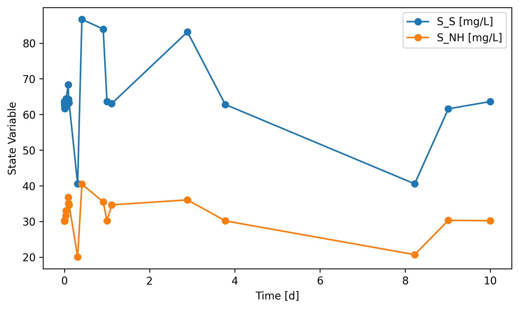
3.2.1. What does DynamicInfluent() default to?

Constructing DI() with no arguments loaded a ready-made BSM1-style influent time series. That’s a real file shipped with QSDsan; we can see it directly.

from qsdsan.unit_operations.dynamic._influent import dynamic_inf_path
print(dynamic_inf_path)
inf_df = pd.read_csv(dynamic_inf_path, sep='\t')
print(f'rows: {len(inf_df)},   columns: {list(inf_df.columns)}')
inf_df.head()

C:\Users\Yalin\Documents\Coding\QSDsan-platform\QSDsan\qsdsan\data\sanunit_data/_inf_dry_2006.tsv
rows: 1345,   columns: ['t', 'S_I', 'S_S', 'X_I', 'X_S', 'X_BH', 'S_NH', 'S_ND', 'X_ND', 'S_ALK', 'Q']

	t	S_I	S_S	X_I	X_S	...	S_NH	S_ND	X_ND	S_ALK	Q
0	0	30	63.6	58.5	224	...	30.2	6.36	11.8	84	21477
1	0.0104	30	61.7	58.5	224	...	30.2	6.17	11.8	84	21474
2	0.0208	30	61.7	53.1	224	...	31	6.17	11.6	84	19620
3	0.0312	30	62.2	51.5	221	...	31.7	6.22	11.4	84	19334
4	0.0417	30	64.6	49.7	218	...	33.2	6.46	11.2	84	18978

5 rows × 11 columns

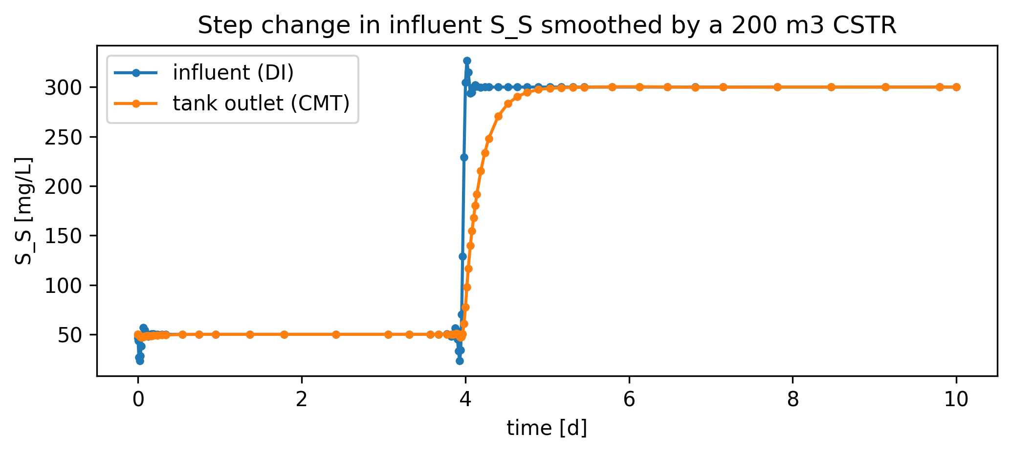
3.2.2. Supplying your own time series

To drive a system with custom influent dynamics, write a CSV with a t column and one column per component (plus Q for total volumetric flow), then pass data_file= to DynamicInfluent. Below we feed a step change in S_S into the same CompleteMixTank from §2.5 and watch the tank smooth the step out.

import matplotlib.pyplot as plt

# Author a 10-day step-change time series: S_S jumps from 50 to 300 mg/L at t=4 d.
custom_path = os.path.join(tmpdir, 'custom_inf.csv')
t_step = np.linspace(0, 10, 201)
S_S_step = np.where(t_step < 4.0, 50.0, 300.0)
custom_df = pd.DataFrame({'t': t_step, 'S_S': S_S_step, 'Q': 1000.0})
custom_df.to_csv(custom_path, index=False)

DI_step = DI(ID='DI_step', outs=('step_inf',), data_file=custom_path)
tank2 = CompleteMixTank(ID='T2', ins=DI_step-0, V=200, isdynamic=True)
tank2.set_init_conc(S_S=50.0)
sys_di2 = qs.System('di_step_sys', path=(DI_step, tank2))
sys_di2.set_dynamic_tracker(DI_step, tank2)
sys_di2.simulate(t_span=(0, 10), method='BDF',
                 t_eval=np.linspace(0, 10, 201),
                 state_reset_hook='reset_cache')

# Both `DI_step.scope` and `tank2.scope` are SanUnitScopes whose `.header`
# entries look like ('id', 'S_S [mg/L]'); split off the units suffix to match
# by component name.
def col(scope, name):
    return next(i for i, h in enumerate(scope.header) if h[1].split()[0] == name)

S_S_in_idx  = col(DI_step.scope, 'S_S')
S_S_out_idx = col(tank2.scope, 'S_S')

t_in    = DI_step.scope.time_series
S_S_in  = DI_step.scope.record[:, S_S_in_idx]
t_out   = tank2.scope.time_series
S_S_out = tank2.scope.record[:, S_S_out_idx]

fig, ax = plt.subplots(figsize=(7, 3.2))
ax.plot(t_in,  S_S_in,  '-o', label='influent (DI)', markersize=3)
ax.plot(t_out, S_S_out, '-o', label='tank outlet (CMT)', markersize=3)
ax.set_ylabel('S_S [mg/L]'); ax.set_xlabel('time [d]')
ax.set_title('Step change in influent S_S smoothed by a 200 m3 CSTR')
ax.legend()
fig.tight_layout()

---

↑ Back to top