Quick Overview
Click the badge below to try this tutorial interactively in your browser:
![]()
You can also run this tutorial inGoogle Colab. It takes a one-time setup per session: follow theColab instructions.
Prepared by:
Learning objectives. After this tutorial, you will be able to:
See how the main
QSDsanclasses (Component,WasteStream,SanUnit,System,TEA,LCA,Process) fit togetherPreview the typical workflow from defining components to running an analysis
Decide which subsequent tutorials to read based on what you want to build
QSDsan is a Python platform for the quantitative sustainable design of sanitation and resource recovery systems. Built on BioSTEAM, it lets you assemble treatment trains as connected unit operations, compute techno-economic and life-cycle impact metrics, and explore uncertainty and sensitivity across designs.
This tutorial is a brief tour of the main pieces. Each class shown here has its own dedicated tutorial; pointers are at the end.
Setup
Import QSDsan and confirm the installed version.
[1]:
import qsdsan as qs, exposan
print(f'This tutorial was made with qsdsan v{qs.__version__} and exposan v{exposan.__version__}')
This tutorial was made with qsdsan v1.5.3 and exposan v1.5.3
1. The pieces of QSDsan
QSDsan groups its functionality into a small set of core classes:
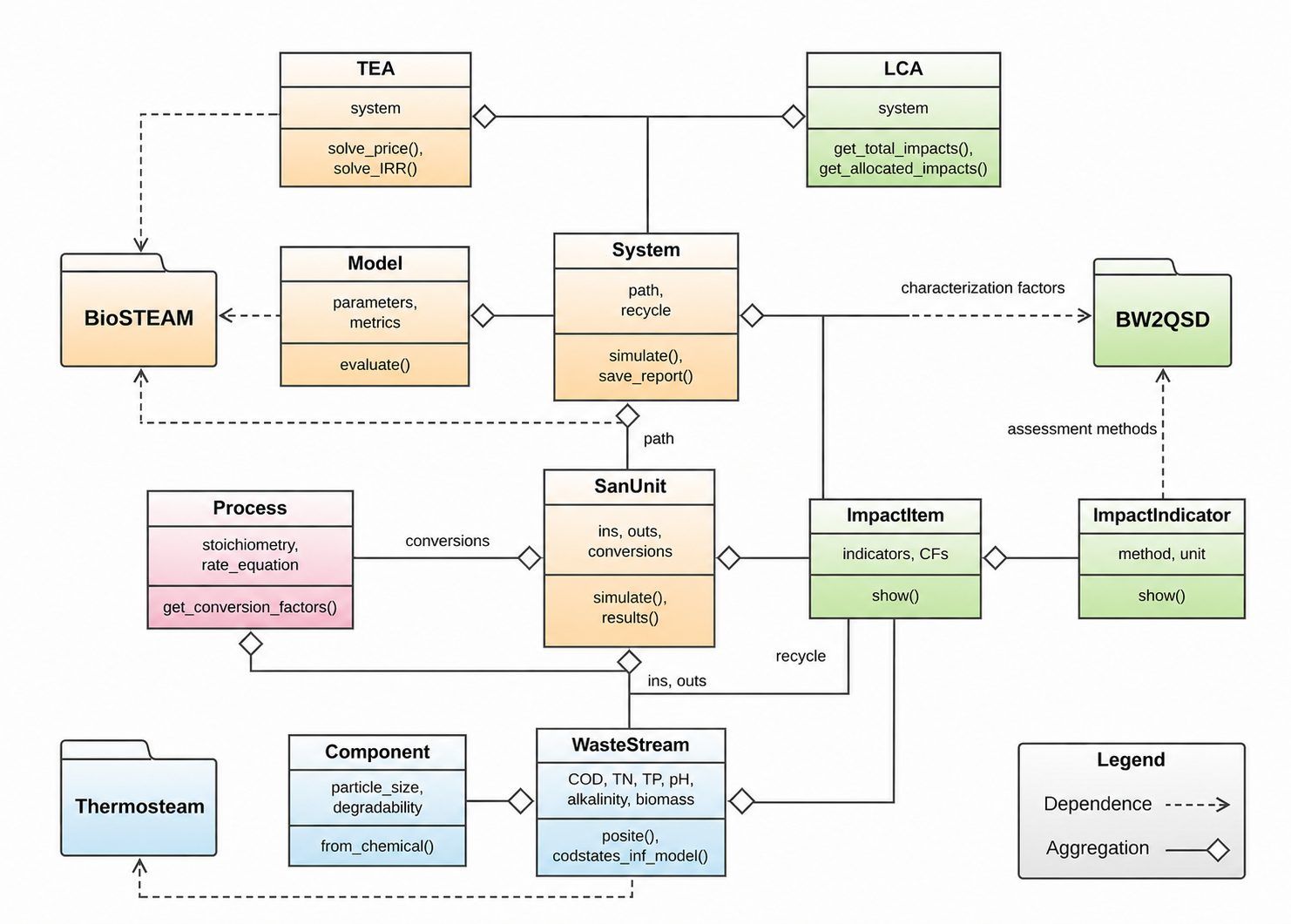
Thermosteam, BioSTEAM, and BW2QSD are external packages that QSDsan leverages.
Class |
What it represents |
|---|---|
|
A chemical or biological species, with thermodynamic and biological properties |
|
A flow of components, with composition and thermodynamic state |
|
A unit operation, with |
|
A connected set of units representing a treatment train |
|
Rate expressions and stoichiometry for dynamic biokinetic models |
|
Techno-economic analysis on a |
|
Life cycle assessment on a |
|
Parameters and metrics for uncertainty and sensitivity analyses |
The rest of this tour shows each one briefly.
2. Components and Streams
A Component describes one species (a chemical, a microbial group, or an aggregate parameter such as COD). A Components registry defines the thermodynamic basis for the model and must be set as the active thermo before building streams. See the Component tutorial for more information.
[2]:
cmps = qs.Components.load_default()
qs.set_thermo(cmps)
cmps.show()
CompiledComponents([
    S_H2,      S_CH4,       S_CH3OH,     S_Ac,
    S_Prop,    S_F,         S_U_Inf,     S_U_E,
    C_B_Subst, C_B_BAP,     C_B_UAP,     C_U_Inf,
    X_B_Subst, X_OHO_PHA,   X_GAO_PHA,   X_PAO_PHA,
    X_GAO_Gly, X_PAO_Gly,   X_OHO,       X_AOO,
    X_NOO,     X_AMO,       X_PAO,       X_MEOLO,
    X_FO,      X_ACO,       X_HMO,       X_PRO,
    X_U_Inf,   X_U_OHO_E,   X_U_PAO_E,   X_Ig_ISS,
    X_MgCO3,   X_CaCO3,     X_MAP,       X_HAP,
    X_HDP,     X_FePO4,     X_AlPO4,     X_AlOH,
    X_FeOH,    X_PAO_PP_Lo, X_PAO_PP_Hi, S_NH4,
    S_NO2,     S_NO3,       S_PO4,       S_K,
    S_Ca,      S_Mg,        S_CO3,       S_N2,
    S_O2,      S_CAT,       S_AN,        H2O,
])
Each component carries a rich set of properties:
[3]:
cmps.S_CH4.show(chemical_info=True)
Component: S_CH4 (phase_ref='g')
[Names]  CAS: 74-82-8
         InChI: CH4/h1H4
         InChI_key: VNWKTOKETHGBQD-U...
         common_name: methane
         iupac_name: ('methane',)
         pubchemid: 297
         smiles: C
         formula: CH4
[Groups] Dortmund: <Empty>
         UNIFAC: <Empty>
         PSRK: <Empty>
         NIST: <Empty>
[Data]   MW: 16.042 g/mol
         Tm: 90.75 K
         Tb: 111.67 K
         Tt: 90.694 K
         Tc: 190.56 K
         Pt: 11696 Pa
         Pc: 4.5992e+06 Pa
         Vc: 9.8628e-05 m^3/mol
         Hf: -74534 J/mol
         S0: 186.3 J/K/mol
         LHV: 8.0257e+05 J/mol
         HHV: 8.9059e+05 J/mol
         Hfus: 940 J/mol
         Sfus: 0
         omega: 0.01142
         dipole: 0 Debye
         similarity_variable: 0.31167
         iscyclic_aliphatic: 0
         combustion: {'CO2': 1, 'O2'...
Component-specific properties:
[Others] measured_as: COD
         description: Dissolved Methane
         particle_size: Dissolved gas
         degradability: Readily
         organic: True
         i_C: 0.18767 g C/g COD
         i_N: 0 g N/g COD
         i_P: 0 g P/g COD
         i_K: 0 g K/g COD
         i_Mg: 0 g Mg/g COD
         i_Ca: 0 g Ca/g COD
         i_mass: 0.25067 g mass/g COD
         i_charge: 0 mol +/g COD
         i_COD: 1 g COD/g COD
         i_NOD: 0 g NOD/g COD
         f_BOD5_COD: 0
         f_uBOD_COD: 0
         f_Vmass_Totmass: 1
         chem_MW: 16.042
QSDsan provides three stream classes in a hierarchy. The Stream class is from Thermosteam (BioSTEAM’s thermodynamic engine), which represents a generic material flow. SanStream adds stream-level life cycle impact functionalit, and WasteStream adds wastewater-modeling functionality on top of SanStream. See this comparison page and
the WasteStream tutorial for more information.
A WasteStream holds component flows plus the thermodynamic state. Several convenience initializers are available; for example, a typical municipal influent can be built from a COD-based model:
[4]:
ww = qs.WasteStream.codbased_inf_model('ww', flow_tot=100)
ww.show()
WasteStream: ww
phase: 'l', T: 298.15 K, P: 101325 Pa
flow (g/hr): S_F        7.5
             S_U_Inf    3.25
             C_B_Subst  4
             X_B_Subst  22.7
             X_U_Inf    5.58
             X_Ig_ISS   5.23
             S_NH4      2.5
             S_PO4      0.8
             S_K        2.8
             S_Ca       14
             S_Mg       5
             S_CO3      12
             S_N2       1.8
             S_CAT      0.3
             S_AN       1.2
             ...        9.96e+04
 WasteStream-specific properties:
  pH         : 7.0
  Alkalinity : 10.0 mmol/L
  COD        : 430.0 mg/L
  BOD        : 249.4 mg/L
  TC         : 265.0 mg/L
  TOC        : 137.6 mg/L
  TN         : 40.0 mg/L
  TP         : 10.0 mg/L
  TK         : 28.0 mg/L
  TSS        : 209.3 mg/L
 Component concentrations (mg/L):
  S_F          75.0
  S_U_Inf      32.5
  C_B_Subst    40.0
  X_B_Subst    226.7
  X_U_Inf      55.8
  X_Ig_ISS     52.3
  S_NH4        25.0
  S_PO4        8.0
  S_K          28.0
  S_Ca         140.0
  S_Mg         50.0
  S_CO3        120.0
  S_N2         18.0
  S_CAT        3.0
  S_AN         12.0
  ...
3. Unit Operations
A SanUnit is a unit operation. QSDsan have many pre-built subclasses (clarifiers, anaerobic digesters, membrane filters, etc.) that are often used for sanitation and resource recovery facilities. You can also subclass SanUnit to model your own; see the basic and advanced tutorials for more information.
[5]:
# A small sample of built-in unit operations
# See the list of unit operations in the documentation for more details:
# https://qsdsan.readthedocs.io/en/latest/api/unit_operations/index.html
ops = sorted(i for i in dir(qs.unit_operations) if not i.startswith('_'))
print(f'qsdsan ships {len(ops)} unit operations. A few examples:')
for o in ops[:10]:
    print(f'  - {o}')
qsdsan ships 132 unit operations. A few examples:
  - A1junction
  - ADM1ptomASM2d
  - ADM1toASM2d
  - ADMjunction
  - ADMtoASM
  - ASM2dtoADM1
  - ASM2dtomADM1
  - ASMtoADM
  - ActivatedSludgeProcess
  - AdiabaticMultiStageVLEColumn
4. Process Models
A Process represents a single reaction defined by a rate expression and component stoichiometry. A Processes instance groups related Process objects into a complete dynamic model such as ASM1, ASM2d, or ADM1. See the Process tutorial for more information.
Note. If your model is steady-state, i.e., flows and unit behavior do not change with time, you do not need Process. It is only needed when you need to capture time-varying behavior. The dynamic-modeling tutorials in Part III cover this in depth.
[6]:
asm1_cmps = qs.process_models.create_asm1_cmps(set_thermo=True)
asm1 = qs.process_models.ASM1()
print(asm1.rate_equations)
                                         rate_equation
aero_growth_hetero  4.0*S_NH*S_O*S_S*X_BH/((S_NH + ...
anox_growth_hetero  0.64*S_NH*S_NO*S_S*X_BH/((S_NH ...
aero_growth_auto    0.5*S_NH*S_O*X_BA/((S_NH + 1.0)...
decay_hetero                                  0.3*X_BH
decay_auto                                   0.05*X_BA
ammonification                          0.05*S_ND*X_BH
hydrolysis          3.0*X_BH*X_S*(0.16*S_NO/((S_NO ...
hydrolysis_N        3.0*X_BH*X_ND*(0.16*S_NO/((S_NO...
5. Assembling Unit Operations into a System
Units connect via influent and effluent streams to form a System. Below is an example from EXPOsan (the companion package of established systems). The bwaise study models sanitation for Bwaise, an unplanned settlement in Kampala, Uganda. See the System tutorial for more information.
[7]:
from exposan import bwaise as bw
bw.load()
bw.sysA.diagram()

Once simulated, you can read per-unit results:
[8]:
print(bw.A2.results())
Pit latrine                                      Units       A2
Design              Number of users per toilet               16
                    Parallel toilets                   2.85e+04
                    Emptying period                 yr      0.8
                    Single pit volume               m3     3.66
                    Single pit area                 m2      0.8
                    Single pit depth                 m     4.57
                    Cement                          kg    2e+07
                    Sand                            kg 9.05e+07
                    Gravel                          kg 3.65e+07
                    Brick                           kg 6.47e+06
                    Plastic                         kg 2.88e+05
                    Steel                           kg 9.58e+05
                    Wood                            m3 5.42e+03
                    Excavation                      m3 1.04e+05
Purchase cost       Total toilets                  USD 1.28e+07
Total purchase cost                                USD 1.28e+07
Utility cost                                    USD/hr        0
Additional OPEX                                 USD/hr     73.1
6. Techno-Economic Analysis and Life Cycle Assessment (TEA/LCA)
A TEA runs the techno-economics on a System; an LCA runs the impact assessment. Both attach to the same System and read its simulation results. See the TEA and LCA tutorials for more information.
[9]:
c = qs.currency
print('For sysA in the Bwaise study:\n')
for attr in ('NPV', 'EAC', 'CAPEX', 'AOC', 'sales', 'net_earnings'):
    uom = c if attr in ('NPV', 'CAPEX') else f'{c}/yr'
    print(f'  - {attr}: {getattr(bw.teaA, attr):,.0f} {uom}')
For sysA in the Bwaise study:

  - NPV: -42,012,131 USD
  - EAC: 6,706,210 USD/yr
  - CAPEX: 31,421,918 USD
  - AOC: 1,844,554 USD/yr
  - sales: 206,017 USD/yr
  - net_earnings: -1,638,537 USD/yr
The LCA object summarizes impacts by category and contributor:
[10]:
bw.lcaA
LCA: sysA (lifetime 8 yr)
Impacts:
                           Construction  Transportation   Stream   Others    Total
GlobalWarming (kg CO2-eq)      3.13e+07        9.57e+05 1.82e+08 5.19e+04 2.14e+08
7. Uncertainty and Sensitivity Analyses
To perform uncertainty and sensitiviy analysis, a Model object is built on a System to add uncertain distributions of the input parameters and define output metrics of interest. The Model object can be then used to run Monte Carlo (for uncertainty) and sensitivity analyses. See the Uncertainty and Sensitivity Analyses for more information.
[11]:
bw.modelA # shows the declared uncertainty parameters
QSDsan also includes a stats module for statistical analysis (e.g., global sensitivity analysis), including and visualization helpers.
Where to go next
The tutorials are organized in three parts. You just finished Part I.
Part II. QSDsan’s core classes. Each tutorial dives into one or a few of the classes you just saw.
Part III. Integrating process models. Build dynamic, multi-component models on top of QSDsan.
↑ Back to top