Anaerobic Digestion Model No. 1 (ADM1)¶

Prepared by:
- Ga-Yeong Kim
Covered topics:
- 1. Introduction
- 2. System Setup
- 3. System Simulation

To run tutorials in your browser, go to this Binder page.

[1]:

import qsdsan as qs, exposan
print(f'This tutorial was made with qsdsan v{qs.__version__} and exposan v{exposan.__version__}')

This tutorial was made with qsdsan v1.3.1 and exposan v1.3.1

1. Introduction¶

Anaerobic Digestion Model No.1 (ADM1) includes multiple steps describing biochemical as well as physicochemical processes.

The biochemical steps include disintegration from homogeneous particulates to carbohydrates, proteins and lipids; extracellular hydrolysis of these particulate substrates to sugars, amino acids, and long chain fatty acids (LCFA), respectively; acidogenesis from sugars and amino acids to volatile fatty acids (VFAs) and hydrogen; acetogenesis of LCFA and VFAs to acetate; and separate methanogenesis steps from acetate and hydrogen/CO2.

The physico-chemical equations describe ion association and dissociation, and gas-liquid transfer.

Implemented as a differential and algebraic equation (DAE) set, there are 26 dynamic state concentration variables, and 8 implicit algebraic variables per reactor vessel or element. Implemented as differential equations (DE) only, there are 32 dynamic concentration state variables.

Water Science and Technology, Vol 45, No 10, pp 65–73

assets/ADM1.JPG

Note: You can find validation of the ADM1 system in EXPOsan.

2. System Setup¶

[2]:

# Import packages
import numpy as np
from chemicals.elements import molecular_weight as get_mw
from qsdsan import sanunits as su, processes as pc, WasteStream, System
from qsdsan.utils import time_printer

import warnings
warnings.simplefilter(action='ignore', category=FutureWarning)        # to ignore Pandas future warning

2.1. State variables of ADM1¶

[3]:

# Components
cmps = pc.create_adm1_cmps()           # create state variables for ADM1
cmps.show()                            # 26 components in ADM1 + water

CompiledComponents([S_su, S_aa, S_fa, S_va, S_bu, S_pro, S_ac, S_h2, S_ch4, S_IC, S_IN, S_I, X_c, X_ch, X_pr, X_li, X_su, X_aa, X_fa, X_c4, X_pro, X_ac, X_h2, X_I, S_cat, S_an, H2O])

S_su: Monosaccharides, S_aa: Amino acids, S_fa: Total long-chain fatty acids, S_va: Total valerate, S_bu: Total butyrate, S_pro: Total propionate, S_ac: Total acetate, S_h2: Hydrogen gas, S_ch4: Methane gas, S_IC: Inorganic carbon, S_IN: Inorganic nitrogen, S_I: Soluble inerts, X_c: Composites, X_ch: Carobohydrates, X_pr: Proteins, X_li: Lipids, X_su: Biomass uptaking sugars, X_aa: Biomass uptaking amino acids, X_fa: Biomass uptaking long chain fatty acids, X_c4: Biomass uptaking c4 fatty acids (valerate and butyrate), X_pro: Biomass uptaking propionate, X_ac: Biomass uptaking acetate, X_h2: Biomass uptaking hydrogen, X_I: Particulate inerts, S_cat: Other cations, S_an: Other anions

2.2. The ADM1 `Process`¶

[4]:

# Processes
adm1 = pc.ADM1()                       # create ADM1 processes
adm1.show()                            # 22 processes in ADM1

ADM1([disintegration, hydrolysis_carbs, hydrolysis_proteins, hydrolysis_lipids, uptake_sugars, uptake_amino_acids, uptake_LCFA, uptake_valerate, uptake_butyrate, uptake_propionate, uptake_acetate, uptake_h2, decay_Xsu, decay_Xaa, decay_Xfa, decay_Xc4, decay_Xpro, decay_Xac, decay_Xh2, h2_transfer, ch4_transfer, IC_transfer])

2.3. Petersen matrix of ADM1¶

[5]:

# Petersen stoichiometric matrix
adm1.stoichiometry

[5]:

	S_su	S_aa	S_fa	S_va	S_bu	...	X_h2	X_I
disintegration	0	0	0	0	0	...	0	0.2
hydrolysis_carbs	1	0	0	0	0	...	0	0
hydrolysis_proteins	0	1	0	0	0	...	0	0
hydrolysis_lipids	0.05	0	0.95	0	0	...	0	0
uptake_sugars	-1	0	0	0	0.117	...	0	0
uptake_amino_acids	0	-1	0	0.212	0.239	...	0	0
uptake_LCFA	0	0	-1	0	0	...	0	0
uptake_valerate	0	0	0	-1	0	...	0	0
uptake_butyrate	0	0	0	0	-1	...	0	0
uptake_propionate	0	0	0	0	0	...	0	0
uptake_acetate	0	0	0	0	0	...	0	0
uptake_h2	0	0	0	0	0	...	0.06	0
decay_Xsu	0	0	0	0	0	...	0	0
decay_Xaa	0	0	0	0	0	...	0	0
decay_Xfa	0	0	0	0	0	...	0	0
decay_Xc4	0	0	0	0	0	...	0	0
decay_Xpro	0	0	0	0	0	...	0	0
decay_Xac	0	0	0	0	0	...	0	0
decay_Xh2	0	0	0	0	0	...	-1	0
h2_transfer	0	0	0	0	0	...	0	0
ch4_transfer	0	0	0	0	0	...	0	0
IC_transfer	0	0	0	0	0	...	0	0

22 rows × 27 columns

The rate of production or consumption for a state variable

\(a_{ij}\): the stoichiometric coefficient of component \(j\) in process \(i\) (i.e., value on the \(i\)th row and \(j\)th column of the stoichiometry matrix) \(\rho_i\): process \(i\)’s reaction rate \(r_j\): the overall production or consumption rate of component \(j\)

\[r_j = \sum_i{a_{ij}\cdot\rho_i}\]

In matrix notation, this calculation can be neatly described as

\[\mathbf{r} = \mathbf{A^T} \mathbf{\rho}\]

where \(\mathbf{A}\) is the stoichiometry matrix and \(\mathbf{\rho}\) is the array of process rates.

2.4. Influent & effluent¶

[6]:

# Flow rate, temperature, HRT
Q = 170                                             # influent flowrate [m3/d]
Temp = 273.15+35                                    # temperature [K]
HRT = 5                                             # HRT [d]

[7]:

# WasteStream
inf = WasteStream('Influent', T=Temp)               # influent
eff = WasteStream('Effluent', T=Temp)               # effluent
gas = WasteStream('Biogas')                         # gas

[8]:

# Set influent concentration
C_mw = get_mw({'C':1})        # molecular weight of carbon
N_mw = get_mw({'N':1})        # molecular weight of nitrogen

default_inf_kwargs = {
    'concentrations': {
        'S_su':0.01,
        'S_aa':1e-3,
        'S_fa':1e-3,
        'S_va':1e-3,
        'S_bu':1e-3,
        'S_pro':1e-3,
        'S_ac':1e-3,
        'S_h2':1e-8,
        'S_ch4':1e-5,
        'S_IC':0.04*C_mw,
        'S_IN':0.01*N_mw,
        'S_I':0.02,
        'X_c':2.0,
        'X_ch':5.0,
        'X_pr':20.0,
        'X_li':5.0,
        'X_aa':1e-2,
        'X_fa':1e-2,
        'X_c4':1e-2,
        'X_pro':1e-2,
        'X_ac':1e-2,
        'X_h2':1e-2,
        'X_I':25,
        'S_cat':0.04,
        'S_an':0.02,
        },
    'units': ('m3/d', 'kg/m3'),
    }                                                           # concentration of each state variable in influent

inf.set_flow_by_concentration(Q, **default_inf_kwargs)          # set influent concentration
inf

WasteStream: Influent
phase: 'l', T: 308.15 K, P: 101325 Pa
flow (g/hr): S_su   70.8
             S_aa   7.08
             S_fa   7.08
             S_va   7.08
             S_bu   7.08
             S_pro  7.08
             S_ac   7.08
             S_h2   7.08e-05
             S_ch4  0.0708
             S_IC   3.4e+03
             S_IN   992
             S_I    142
             X_c    1.42e+04
             X_ch   3.54e+04
             X_pr   1.42e+05
             ...    6.97e+06
 WasteStream-specific properties:
  pH         : 7.0
  Alkalinity : 2.5 mg/L
  COD        : 57096.0 mg/L
  BOD        : 12769.4 mg/L
  TC         : 20596.5 mg/L
  TOC        : 20116.0 mg/L
  TN         : 3683.2 mg/L
  TP         : 489.3 mg/L
  TK         : 9.8 mg/L
 Component concentrations (mg/L):
  S_su   10.0
  S_aa   1.0
  S_fa   1.0
  S_va   1.0
  S_bu   1.0
  S_pro  1.0
  S_ac   1.0
  S_h2   0.0
  S_ch4  0.0
  S_IC   480.4
  S_IN   140.1
  S_I    20.0
  X_c    2000.0
  X_ch   5000.0
  X_pr   20000.0
  ...

2.5. Reactor¶

[9]:

# SanUnit
AD = su.AnaerobicCSTR('AD', ins=inf, outs=(gas, eff), model=adm1, V_liq=Q*HRT, V_gas=Q*HRT*0.1, T=Temp)

su.AnaerobicCSTR( ID=’’, ins=None, outs=(), thermo=None, init_with=’WasteStream’, V_liq=3400, V_gas=300, model=None, T=308.15, headspace_P=1.013, external_P=1.013, pipe_resistance=50000.0, fixed_headspace_P=False, retain_cmps=(), fraction_retain=0.95, isdynamic=True, exogenous_vars=(), **kwargs, )

Parameters ins : :class:WasteStream, Influent to the reactor. outs : Iterable, Biogas and treated effluent(s). V_liq : float, optional, Liquid-phase volume [m^3]. The default is 3400. V_gas : float, optional, Headspace volume [m^3]. The default is 300. model : :class:Processes, optional, The kinetic model, typically ADM1-like. The default is None. T : float, optional, Operation temperature [K]. The default is 308.15. headspace_P : float, optional, Headspace pressure, if fixed [bar]. The default is 1.013. external_P : float, optional, External pressure, typically atmospheric pressure [bar]. The default is 1.013. pipe_resistance : float, optional, Biogas extraction pipe resistance [m3/d/bar]. The default is 5.0e4. fixed_headspace_P : bool, optional, Whether to assume fixed headspace pressure. The default is False. retain_cmps : Iterable[str], optional, IDs of the components that are assumed to be retained in the reactor, ideally. The default is (). fraction_retain : float, optional, The assumed fraction of ideal retention of select components. The default is 0.95.

[10]:

AD                                                             # anaerobic CSTR with influent, effluent, and biogas
                                                               # before running the simulation, 'outs' have nothing

../_images/tutorials_12_Anaerobic_Digestion_Model_No_1_23_0.svg

AnaerobicCSTR: AD
ins...
[0] Influent
phase: 'l', T: 308.15 K, P: 101325 Pa
flow (g/hr): S_su   70.8
                S_aa   7.08
                S_fa   7.08
                S_va   7.08
                S_bu   7.08
                S_pro  7.08
                S_ac   7.08
                S_h2   7.08e-05
                S_ch4  0.0708
                S_IC   3.4e+03
                S_IN   992
                S_I    142
                X_c    1.42e+04
                X_ch   3.54e+04
                X_pr   1.42e+05
                ...    6.97e+06
    WasteStream-specific properties:
     pH         : 7.0
     COD        : 57096.0 mg/L
     BOD        : 12769.4 mg/L
     TC         : 20596.5 mg/L
     TOC        : 20116.0 mg/L
     TN         : 3683.2 mg/L
     TP         : 489.3 mg/L
     TK         : 9.8 mg/L
outs...
[0] Biogas
phase: 'l', T: 298.15 K, P: 101325 Pa
flow: 0
    WasteStream-specific properties: None for empty waste streams
[1] Effluent
phase: 'l', T: 308.15 K, P: 101325 Pa
flow: 0
    WasteStream-specific properties: None for empty waste streams

[11]:

# Set initial condition of the reactor
default_init_conds = {
    'S_su': 0.0124*1e3,
    'S_aa': 0.0055*1e3,
    'S_fa': 0.1074*1e3,
    'S_va': 0.0123*1e3,
    'S_bu': 0.0140*1e3,
    'S_pro': 0.0176*1e3,
    'S_ac': 0.0893*1e3,
    'S_h2': 2.5055e-7*1e3,
    'S_ch4': 0.0555*1e3,
    'S_IC': 0.0951*C_mw*1e3,
    'S_IN': 0.0945*N_mw*1e3,
    'S_I': 0.1309*1e3,
    'X_ch': 0.0205*1e3,
    'X_pr': 0.0842*1e3,
    'X_li': 0.0436*1e3,
    'X_su': 0.3122*1e3,
    'X_aa': 0.9317*1e3,
    'X_fa': 0.3384*1e3,
    'X_c4': 0.3258*1e3,
    'X_pro': 0.1011*1e3,
    'X_ac': 0.6772*1e3,
    'X_h2': 0.2848*1e3,
    'X_I': 17.2162*1e3
    }                                                           # concentration of each state variable in reactor

AD.set_init_conc(**default_init_conds)                          # set initial condition of AD

2.6. System set-up¶

[12]:

# System
sys = System('Anaerobic_Digestion', path=(AD,))                 # aggregation of sanunits
sys.set_dynamic_tracker(eff, gas)                               # what you want to track changes in concentration
sys                                                             # before running the simulation, 'outs' have nothing

../_images/tutorials_12_Anaerobic_Digestion_Model_No_1_26_0.svg

System: Anaerobic_Digestion
ins...
[0] Influent
    phase: 'l', T: 308.15 K, P: 101325 Pa
    flow (kmol/hr): S_su   0.000393
                    S_aa   0.00708
                    S_fa   2.76e-05
                    S_va   6.94e-05
                    S_bu   8.13e-05
                    S_pro  9.69e-05
                    S_ac   0.00012
                    ...    709
outs...
[0] Biogas
    phase: 'l', T: 298.15 K, P: 101325 Pa
    flow: 0
[1] Effluent
    phase: 'l', T: 308.15 K, P: 101325 Pa
    flow: 0

3. System Simulation¶

[13]:

# Simulation settings
t = 10                          # total time for simulation
t_step = 0.1                    # times at which to store the computed solution

method = 'BDF'                  # integration method to use
# method = 'RK45'
# method = 'RK23'
# method = 'DOP853'
# method = 'Radau'
# method = 'LSODA'

# https://docs.scipy.org/doc/scipy/reference/generated/scipy.integrate.solve_ivp.html

[14]:

# Run simulation
sys.simulate(state_reset_hook='reset_cache',
             t_span=(0,t),
             t_eval=np.arange(0, t+t_step, t_step),
             method=method,
            # export_state_to=f'sol_{t}d_{method}_AD.xlsx',               # uncomment to export simulation result as excel file
            )

[15]:

sys                                                                      # now you have 'outs' info.

../_images/tutorials_12_Anaerobic_Digestion_Model_No_1_31_0.svg

System: Anaerobic_Digestion
ins...
[0] Influent
    phase: 'l', T: 308.15 K, P: 101325 Pa
    flow (kmol/hr): S_su   0.000393
                    S_aa   0.00708
                    S_fa   2.76e-05
                    S_va   6.94e-05
                    S_bu   8.13e-05
                    S_pro  9.69e-05
                    S_ac   0.00012
                    ...    709
outs...
[0] Biogas
    phase: 'g', T: 308.15 K, P: 101325 Pa
    flow (kmol/hr): S_h2   0.00119
                    S_ch4  8.5
                    S_IC   0.414
                    H2O    0.205
[1] Effluent
    phase: 'l', T: 308.15 K, P: 101325 Pa
    flow (kmol/hr): S_su   0.00164
                    S_aa   0.129
                    S_fa   0.0222
                    S_va   0.00332
                    S_bu   0.00447
                    S_pro  0.0106
                    S_ac   0.639
                    ...    587

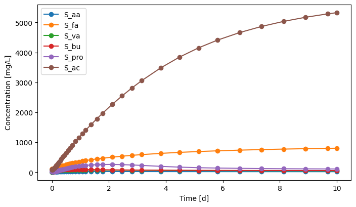
3.1. Check simulation results: Effluent¶

[16]:

eff.scope.plot_time_series(('S_aa', 'S_fa', 'S_va', 'S_bu', 'S_pro', 'S_ac'))  # you can plot how each state variable changes over time

[16]:

(<Figure size 800x450 with 1 Axes>,
 <Axes: xlabel='Time [d]', ylabel='Concentration [mg/L]'>)

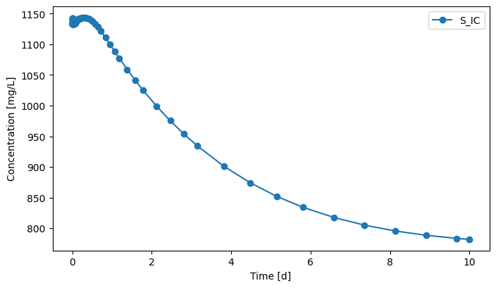
../_images/tutorials_12_Anaerobic_Digestion_Model_No_1_33_1.png

[17]:

eff.scope.plot_time_series(('S_IC'))

[17]:

(<Figure size 800x450 with 1 Axes>,
 <Axes: xlabel='Time [d]', ylabel='Concentration [mg/L]'>)

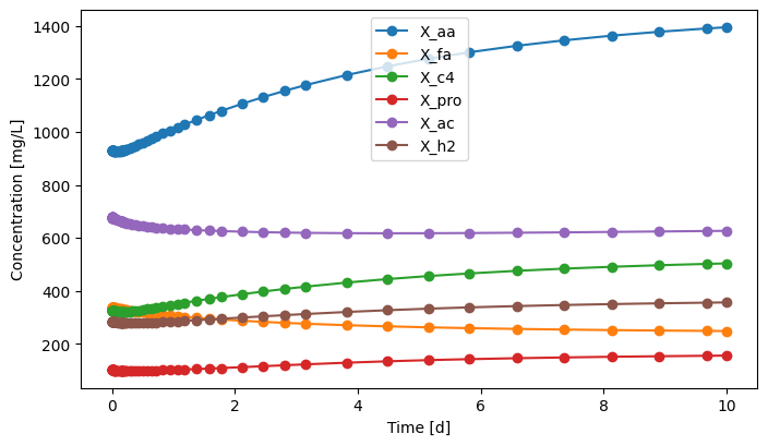
../_images/tutorials_12_Anaerobic_Digestion_Model_No_1_34_1.png

[18]:

eff.scope.plot_time_series(('X_aa', 'X_fa', 'X_c4', 'X_pro', 'X_ac', 'X_h2'))

[18]:

(<Figure size 800x450 with 1 Axes>,
 <Axes: xlabel='Time [d]', ylabel='Concentration [mg/L]'>)

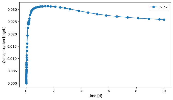
../_images/tutorials_12_Anaerobic_Digestion_Model_No_1_35_1.png

3.2. Check simulation results: Gas¶

[19]:

gas.scope.plot_time_series(('S_h2'))

[19]:

(<Figure size 800x450 with 1 Axes>,
 <Axes: xlabel='Time [d]', ylabel='Concentration [mg/L]'>)

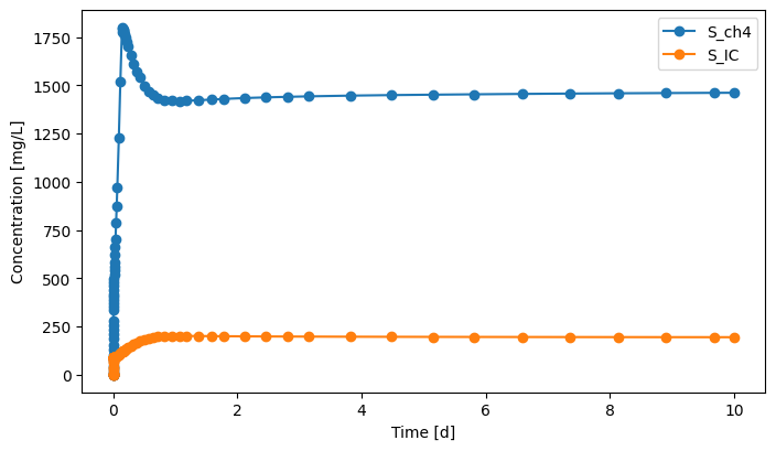
../_images/tutorials_12_Anaerobic_Digestion_Model_No_1_37_1.png

[20]:

gas.scope.plot_time_series(('S_ch4','S_IC'))

[20]:

(<Figure size 800x450 with 1 Axes>,
 <Axes: xlabel='Time [d]', ylabel='Concentration [mg/L]'>)

../_images/tutorials_12_Anaerobic_Digestion_Model_No_1_38_1.png

3.3. Check simulation results: Total VFAs¶

[21]:

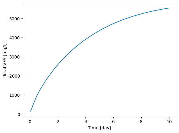
# Total VFAs = 'S_va' + 'S_bu' + 'S_pro' + 'S_ac'    (you can change the equations based on your assumption)
idx_vfa = cmps.indices(['S_va', 'S_bu', 'S_pro', 'S_ac'])

t_stamp = eff.scope.time_series

vfa = eff.scope.record[:,idx_vfa]
total_vfa = np.sum(vfa, axis=1)

[22]:

import matplotlib.pyplot as plt
plt.plot(t_stamp, total_vfa)
plt.xlabel("Time [day]")
plt.ylabel("Total VFA [mg/l]")

[22]:

Text(0, 0.5, 'Total VFA [mg/l]')

../_images/tutorials_12_Anaerobic_Digestion_Model_No_1_41_1.png