Dynamic Simulation
Prepared by:
Covered topics:
1. Understanding dynamic simulation with QSDsan
2. Writing a dynamic SanUnit
3. Other convenient features
Video demo:
To run tutorials in your browser, go to this Binder page.
You can also watch a video demo on YouTube (subscriptions & likes appreciated!).
From previous tutorials, we’ve covered how to use QSDsan’s SanUnit and WasteStream classes to model the mass/energy flows throughout a system. You may have noticed, the simulation results generated by SanUnit._run are static, i.e., they don’t carry time-related information.
In this tutorial, we will learn about the dynamic simulation features in QSDsan. First we will focus on performing dynamic simulations with an existing system to understand the basics. Then we’ll go over how to implement your own algorithms for dynamic simulations.
[1]:
import qsdsan as qs, exposan
print(f'This tutorial was made with qsdsan v{qs.__version__} and exposan v{exposan.__version__}')
This tutorial was made with qsdsan v1.3.1 and exposan v1.3.1
1. Understanding dynamic simulation with QSDsan
1.1. An example system
Let’s use Benchmark Simulation Model no.1 (BSM1) as an example. BSM1 describes an activated sludge treatment process that can be commonly found in conventional wastewater treatment facilities. The full system has been implemented in EXPOsan.
The activated sludge process is often characterized as a series of biokinetic reactions in parallel (recap on Process here). The mathematical models of this kind cannot output mass flows or concentrations directly as a function of input. But rather, they describe the rates of change in state variables at any time as a function of the state variables (often concentrations). As a result, simulation of such systems involves
solving a series of ordinary differential equations (ODEs). We have developed features in QSDsan for this specific purpose.
1.1.1. Running dynamic simulation
[2]:
# Let's load the BSM1 system first
from exposan import bsm1
bsm1.load()
sys = bsm1.sys
sys.show()
System: bsm1_sys
ins...
[0] wastewater
    phase: 'l', T: 293.15 K, P: 101325 Pa
    flow (kmol/hr): S_I   23.1
                    S_S   53.4
                    X_I   39.4
                    X_S   155
                    X_BH  21.7
                    S_NH  1.34
                    S_ND  0.381
                    ...   4.26e+04
outs...
[0] effluent
    phase: 'l', T: 293.15 K, P: 101325 Pa
    flow: 0
[1] WAS
    phase: 'l', T: 293.15 K, P: 101325 Pa
    flow: 0
[3]:
# The BSM1 system is composed of 5 CSTRs in series,
# followed by a flat-bottom circular clarifier.
# sys.units
sys.diagram()

[4]:
# If we try to simulate it like we'd do for a "static" system
# sys.simulate()
We run into this error because QSDsan (essentially biosteam in the background) considers this system dynamic, and additional arguments are required for simulate to work.
[5]:
# We can verify that by
sys.isdynamic
[5]:
True
[6]:
# This is because the system contains at least one dynamic SanUnit
# {u: u.isdynamic for u in sys.units}

# If we disable dynamic simulation, then `simulate` would work as usual
sys.isdynamic = False
sys.simulate()
To perform a dynamic simulation of the system, we need to provide at least one additional keyword argument, i.e., t_span, as suggested in the error message. t_span is a 2-tuple indicating the simulation period.
Note: Whether
t_span = (0,10)means 0-10 days or 0-10 hours/minutes/months depends entirely on units of the parameters in the system’s ODEs. For BSM1, it’d mean 0-10 days because all parameters in the ODEs express time in the unit of “day”.
Other often-used keyword arguments include:
t_eval: a 1d array to specify the output time pointsmethod: a string specifying the ODE solverstate_reset_hook: specifies how to reset the simulation
t_span, t_eval, and method are essentially passed to scipy.integrate.solve_ivp function as keyword arguments. See documentation for a complete list of keyword arguments. You may notice that scipy.integrate.solve_ivp also requires input of fun (i.e., the ODEs) and y0 (i.e., the initial
condition). We’ll learn later how System.simulate automates the compilation of these inputs.
[7]:
# Let's try simulating the BSM1 system from day 0 to day 50
# user shorter time or try changing method to 'RK23' (explicit solver) if it takes a long time
sys.isdynamic = True
sys.simulate(t_span=(0, 50), method='BDF', state_reset_hook='reset_cache')
sys.show()
System: bsm1_sys
Highest convergence error among components in recycle
streams {C1-1, O3-0} after 5 loops:
- flow rate   1.46e-11 kmol/hr (4.2e-14%)
- temperature 0.00e+00 K (0%)
ins...
[0] wastewater
    phase: 'l', T: 293.15 K, P: 101325 Pa
    flow (kmol/hr): S_I   23.1
                    S_S   53.4
                    X_I   39.4
                    X_S   155
                    X_BH  21.7
                    S_NH  1.34
                    S_ND  0.381
                    ...   4.26e+04
outs...
[0] effluent
    phase: 'l', T: 293.15 K, P: 101325 Pa
    flow (kmol/hr): S_I   22.6
                    S_S   0.67
                    X_I   3.3
                    X_S   0.142
                    X_BH  7.36
                    X_BA  0.43
                    X_P   1.3
                    ...   4.17e+04
[1] WAS
    phase: 'l', T: 293.15 K, P: 101325 Pa
    flow (kmol/hr): S_I   0.481
                    S_S   0.0143
                    X_I   36
                    X_S   1.55
                    X_BH  80.3
                    X_BA  4.69
                    X_P   14.1
                    ...   884
1.1.2. Retrieve dynamic simulation data
The show method only displays the system’s state at the end of the simulation period. How do we retrieve information on system dynamics? QSDsan uses Scope objects to keep track of values of state variables during simulation.
[8]:
# This shows the units/streams whose state variables are kept track of
# during dynamic simulations.
sys.scope.subjects
[8]:
(<CSTR: A1>, <WasteStream: effluent>)
[9]:
# We see that A1 and effluent are tracked, so we can retrieve their
# time series data through their `scope` attribute, which stores a
# `SanUnitScope` or `WasteStreamScope` object
A1 = sys.flowsheet.unit.A1
A1.scope
# eff = sys.flowsheet.stream.effluent
# eff.scope
[9]:
<SanUnitScope: A1>
[10]:
# `Scope` objects include a function for convenient visualization of time-series data
fig, ax = A1.scope.plot_time_series(('S_NH', 'S_S'))

[11]:
# Raw time-series data are stored in
# A1.scope.record
A2 = sys.flowsheet.unit.A2
A2.scope
A2.scope.record
[11]:
array([], shape=(0, 1), dtype=float64)
Each row in the record attribute is values of A1’s state variables at a certain time point.
[12]:
# This stores the time data
A1.scope.time_series
[12]:
array([0.000e+00, 5.096e-10, 1.019e-09, 6.115e-09, 1.121e-08, 6.217e-08,
       1.131e-07, 3.165e-07, 5.198e-07, 7.231e-07, 1.403e-06, 2.082e-06,
       2.762e-06, 8.671e-06, 1.458e-05, 2.049e-05, 3.168e-05, 4.286e-05,
       5.405e-05, 6.524e-05, 1.049e-04, 1.446e-04, 1.842e-04, 2.239e-04,
       3.090e-04, 3.941e-04, 4.793e-04, 5.644e-04, 6.495e-04, 8.358e-04,
       1.022e-03, 1.208e-03, 1.395e-03, 1.581e-03, 1.767e-03, 2.185e-03,
       2.602e-03, 2.895e-03, 3.189e-03, 3.398e-03, 3.567e-03, 3.736e-03,
       3.905e-03, 4.038e-03, 4.171e-03, 4.304e-03, 4.438e-03, 4.571e-03,
       4.704e-03, 4.849e-03, 4.993e-03, 5.138e-03, 5.283e-03, 5.427e-03,
       5.572e-03, 5.832e-03, 6.093e-03, 6.353e-03, 6.613e-03, 6.874e-03,
       7.332e-03, 7.790e-03, 8.248e-03, 8.706e-03, 9.407e-03, 1.011e-02,
       1.081e-02, 1.151e-02, 1.273e-02, 1.396e-02, 1.519e-02, 1.641e-02,
       1.848e-02, 2.055e-02, 2.195e-02, 2.335e-02, 2.476e-02, 2.616e-02,
       2.857e-02, 3.097e-02, 3.218e-02, 3.338e-02, 3.458e-02, 3.578e-02,
       3.699e-02, 3.949e-02, 4.116e-02, 4.283e-02, 4.450e-02, 4.616e-02,
       5.025e-02, 5.433e-02, 5.842e-02, 6.250e-02, 6.937e-02, 7.624e-02,
       7.709e-02, 7.795e-02, 7.881e-02, 7.967e-02, 8.006e-02, 8.045e-02,
       8.084e-02, 8.182e-02, 8.280e-02, 8.378e-02, 8.420e-02, 8.462e-02,
       8.503e-02, 8.548e-02, 8.593e-02, 8.620e-02, 8.646e-02, 8.712e-02,
       8.778e-02, 9.300e-02, 9.822e-02, 1.096e-01, 1.110e-01, 1.124e-01,
       1.138e-01, 1.144e-01, 1.150e-01, 1.156e-01, 1.171e-01, 1.185e-01,
       1.200e-01, 1.208e-01, 1.216e-01, 1.224e-01, 1.229e-01, 1.233e-01,
       1.236e-01, 1.239e-01, 1.255e-01, 1.262e-01, 1.270e-01, 1.328e-01,
       1.386e-01, 1.519e-01, 1.652e-01, 1.668e-01, 1.685e-01, 1.702e-01,
       1.717e-01, 1.733e-01, 1.842e-01, 1.856e-01, 1.870e-01, 1.878e-01,
       1.886e-01, 1.891e-01, 1.896e-01, 1.899e-01, 1.902e-01, 1.933e-01,
       1.965e-01, 2.170e-01, 2.375e-01, 2.581e-01, 2.592e-01, 2.603e-01,
       2.614e-01, 2.723e-01, 2.832e-01, 3.164e-01, 3.496e-01, 3.828e-01,
       4.503e-01, 5.178e-01, 5.852e-01, 6.527e-01, 7.282e-01, 8.037e-01,
       8.791e-01, 9.546e-01, 1.105e+00, 1.256e+00, 1.406e+00, 1.557e+00,
       1.810e+00, 2.063e+00, 2.317e+00, 2.570e+00, 3.003e+00, 3.436e+00,
       3.869e+00, 4.302e+00, 4.915e+00, 5.528e+00, 6.142e+00, 6.755e+00,
       7.995e+00, 9.236e+00, 1.048e+01, 1.172e+01, 1.341e+01, 1.511e+01,
       1.680e+01, 1.850e+01, 2.118e+01, 2.386e+01, 2.654e+01, 2.923e+01,
       3.427e+01, 3.932e+01, 4.437e+01, 4.942e+01, 5.000e+01])
The tracked time-series data can be exported to a file in two ways.
[13]:
# sys.scope.export('bsm1_time_series.xlsx')

# or

# import numpy as np
# sys.simulate(state_reset_hook='reset_cache',
#              t_span=(0, 50),
#              t_eval=np.arange(0, 51, 1),
#              method='BDF',
#              export_state_to=('bsm1_time_series.xlsx'))
We can also (re-)define which unit or stream to track during dynamic simulation.
[14]:
# Let's say we want to track the clarifier and the waste activated sludge
C1 = sys.flowsheet.unit.C1
WAS = sys.flowsheet.stream.WAS
sys.set_dynamic_tracker(C1, WAS)
sys.scope.subjects
[14]:
(<FlatBottomCircularClarifier: C1>, <WasteStream: WAS>)
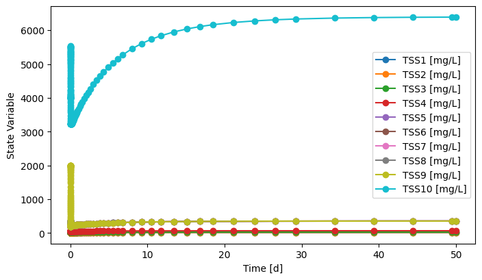
[15]:
# Need to rerun the simulation before retrieving results
# user shorter time or try changing method to 'RK23' (explicit solver) if it takes a long time
sys.simulate(t_span=(0, 50), method='BDF', state_reset_hook='reset_cache')
fig, ax = C1.scope.plot_time_series([f'TSS{i}' for i in range(1,11)])
[16]:
fig, ax = WAS.scope.plot_time_series(('X_BH', 'X_BA'))

So far we’ve learned how to simulate any dynamic system developed with QSDsan. A complete list of existing unit operations within QSDsan is available here. The column “Dynamic” indicates whether the unit is enabled for dynamic simulations. Any system composed of the enabled units can be simulated dynamically as we learned above.
Back to top
1.2. When is a system “dynamic”?
It’s ultimately the user’s decision whether a system should be run dynamically. This section will cover the essentials to switch to the dynamic mode for system simulation.
System.isdynamic vs. SanUnit.isdynamic vs. SanUnit.hasode
Simply speaking, when the
<System>.isdynamic == True, the program will attempt dynamic simulation. Users can directly enable/disable the dynamic mode by setting theisdynamicproperty of aSystemobject.The program will set the value of
<System>.isdynamicwhen it’s not specified by users.<System>.isdynamicis consideredTruein all cases except when<SanUnit>.isdynamic == Falsefor all units.Setting
<SanUnit>.isdynamic = Truedoes not gaurantee the unit can be simulated dynamically. Just like how the_runmethod must be defined for static simulation, a series of additional methods must be defined to enable dynamic simulation.<SanUnit>.hasode == Truemeans a unit has the fundamental methods to compile ODEs. It is a sufficient but not necessary condition for dynamic simulation, because a unit doesn’t have to be described with ODEs to be capable of dynamic simulations.
[17]:
# All units in the BSM1 system above have ODEs
{u: u.hasode for u in sys.units}
[17]:
{<CSTR: A1>: True,
 <CSTR: A2>: True,
 <CSTR: O1>: True,
 <CSTR: O2>: True,
 <CSTR: O3>: True,
 <FlatBottomCircularClarifier: C1>: True}
Back to top
2. Writing a dynamic SanUnit
Whether a system can be simulated dynamically ultimately boils down to whether all the units in the system have the fundamental methods required for dynamic simulations. In this section, you’ll learn how to implement your own algorithms to create a SanUnit subclass capable of dynamic simulations.
2.1. Basic structure
During typical system simulations, _run directly defines the static mass and/or energy flows of the effluent WasteStream objects of the unit after calculation.
In comparison, during dynamic simulations, all information are stored as _state and _dstate attributes of the relevant SanUnit obejcts as well as state and dstate properties of WasteStream objects. These information won’t be translated to mass or energy flows until dynamic simulation is completed.
WasteStream.stateis a 1dnumpy.arrayof length \(n+1\), \(n\) is the length of the components associated with thethermo. Each element of the array represents value of one state variable.
WasteStrem.dstateis an array of the exact same shape asWasteStream.state, storing values of the time derivatives (i.e., the rates of change) of the state variables.
[18]:
sf = sys.flowsheet.stream
sf.effluent.state
[18]:
array([3.000e+01, 8.899e-01, 4.389e+00, 1.886e-01, 9.784e+00, 5.720e-01,
       1.722e+00, 4.897e-01, 1.038e+01, 1.747e+00, 6.884e-01, 1.349e-02,
       4.954e+01, 2.751e+01, 9.978e+05, 1.806e+04])
[19]:
# sf.effluent.F_vol*24  # convert unit from m3/hr to m3/d
sf.effluent.conc
[19]:
sparse([3.000e+01, 8.899e-01, 4.389e+00, 1.886e-01, 9.784e+00, 5.720e-01,
        1.722e+00, 4.897e-01, 1.038e+01, 1.747e+00, 6.884e-01, 1.349e-02,
        4.954e+01, 2.751e+01, 9.981e+05])
[20]:
sf.effluent.dstate.shape == sf.effluent.state.shape
[20]:
True
SanUnit._stateis also a 1dnumpy.array, but the length of the array is not assumed, because the state variables relevant for aSanUnitis entirely dependent on the unit operation itself. Therefore, there is no predefined units of measure or order for state variables of a unit operation.SanUnit._dstate, similarly, must have the exact same shape as the_statearray, as each element corresponds to the time derivative of a state variable.
[21]:
C1._state.shape == A1._state.shape
# C1._state.shape == C1._dstate.shape
[21]:
False
[22]:
# Some dynamic units in QSDsan have a `state` property that formats
# the data in `_state` for better readability
A1.state
[22]:
{'S_I': 30.0,
 'S_S': 2.8098296544615704,
 'X_I': 1147.8970757884535,
 'X_S': 82.14996504835973,
 'X_BH': 2551.1712941951987,
 'X_BA': 148.18576250649838,
 'X_P': 447.1086242830684,
 'S_O': 0.004288622012845044,
 'S_NO': 5.33892893863284,
 'S_NH': 7.928812844268634,
 'S_ND': 1.216680910568711,
 'X_ND': 5.285760801254182,
 'S_ALK': 59.158219028756534,
 'S_N2': 25.008073542375985,
 'H2O': 997794.331078558,
 'Q': 92229.99999999996}
Back to top
2.2. Fundamental methods
In addition to proper __init__ and _run methods (recap), a few more methods are required in a SanUnit subclass for dynamic simulation. Users typically won’t interact with these methods but they will be called by System.simulate to manipulate the values of the arrays mentioned above (i.e., <SanUnit>._state, <SanUnit>._dstate, <WasteStream>.state, and
<WasteStream>.dstate).
_init_state, called after_runto generate an initial condition for the unit, i.e., defining shape and values of the_stateand_dstatearrays. For example:
import numpy as np
def _init_state(self):
    inf = self.ins[0]
    self._state = np.ones(len(inf.components)+1)
    self._dstate = self._state * 0.
This method (not saying it makes sense) assumes \(n+1\) state variables and gives an initial value of 1 to all of them. Then it also sets the initial time derivatives to be 0.
_update_state, to update effluent streams’ state arrays based on current state (and maybe dstate) of the SanUnit. For example:
def _update_state(self):
    arr = self._state   # retrieving the current state of the SanUnit
    eff, = self.outs    # assuming this SanUnit has one outlet only
    eff.state[:] = arr  # assume arr has the same shape as WasteStream.state
The goal of this method is to update the values in <WasteStream>.state for each WasteStream in <SanUnit>.outs.
_update_dstate, to update effluent streams’dstatearrays based on current_stateand_dstateof the SanUnit. The signiture and often the algorithm are similar to_update_state._compile_ODEor_compile_AE, used to define the function that updates the_dstateand/or_stateof theSanUnitbased on its influent streams’state/dstateand potentially its own current state. The defined function will be stored asSanUnit._ODEorSanUnit._AE. These methods should follow some general forms like below:
@property
def ODE(self):
    if self._ODE is None:
        self._compile_ODE()
    return self._ODE
def _compile_ODE(self):
    _dstate = self._dstate
    _update_dstate = self._update_dstate
    def dy_dt(t, y_ins, y, dy_ins):
        _dstate[:] = some_algorithm(t, y_ins, y, dy_ins)
        _update_dstate()
    self._ODE = dy_dt
@property
def AE(self):
    if self._AE is None:
        self._compile_AE()
    return self._AE
def _compile_AE(self):
    _state = self._state
    _dstate = self._dstate
    _update_state = self._update_state
    _update_dstate = self._update_dstate
    def y_t(t, y_ins, dy_ins):
        _state[:] = some_algorithm(t, y_ins, dy_ins)
        _dstate[:] = some_other_algorithm(t, y_ins, dy_ins)
        _update_state()
        _update_dstate()
    self._AE = y_t
Note: Within the
dy_dtory_tfunctions,<SanUnit>._state[:] = <new_value>rather than<SanUnit>._state = <new_value>because it’s generally faster to update values in an existing array than overwriting this array with a newly created array.
We’ll learn more about these two methods in the next subsections.
Back to top
2.3. Making a simple MixerSplitter (_compile_AE)
Let’s say we want to make an ideal mixer-splitter that instantly mixes all streams at the inlets and then evenly split them across the outlets.
[23]:
# Typically if implemented as a static SanUnit, it'd be pretty simple
# Let's ignore `_design` and `_cost` for now.
class MixerSplitter1(qs.SanUnit):
    _N_outs = 3
    _ins_size_is_fixed = False
    _outs_size_is_fixed = False
    def __init__(self, ID='', ins=None, outs=(), thermo=None,
                 init_with='WasteStream', **kwargs):
        qs.SanUnit.__init__(self, ID, ins, outs, thermo, init_with, **kwargs)
        self.mixed = qs.WasteStream()

    def _run(self):
        mixed = self.mixed
        mixed.mix_from(self.ins)
        n_outs = len(self.outs)
        flow = mixed.get_total_flow('kg/hr')/n_outs
        for out in self.outs:
            out.copy_like(mixed)
            out.set_total_flow(flow, 'kg/hr')

    def _design(self):
        pass

    def _cost(self):
        pass
[24]:
# Let's try simulating it with the components used in BSM1
cmps = qs.get_thermo().chemicals
cmps.show()
CompiledComponents([S_I, S_S, X_I, X_S, X_BH, X_BA, X_P, S_O, S_NO, S_NH, S_ND, X_ND, S_ALK, S_N2, H2O])
[25]:
# Now let's make a couple fake influents
inf1 = qs.WasteStream(H2O=1000, S_O=5)
inf2 = qs.WasteStream(H2O=800, S_S=3, S_NH=2.1)
inf2.show()
WasteStream: ws12
phase: 'l', T: 298.15 K, P: 101325 Pa
flow (g/hr): S_S   3e+03
             S_NH  2.1e+03
             H2O   8e+05
 WasteStream-specific properties:
  pH         : 7.0
  Alkalinity : 2.5 mg/L
  COD        : 3711.8 mg/L
  BOD        : 2661.3 mg/L
  TC         : 1187.8 mg/L
  TOC        : 1187.8 mg/L
  TN         : 2598.2 mg/L
  TP         : 37.1 mg/L
 Component concentrations (mg/L):
  S_S    3711.8
  S_NH   2598.2
  H2O    989803.5
[26]:
MS1 = MixerSplitter1(ins=(inf1, inf2))
MS1.simulate()
MS1.show()
MixerSplitter1: M1
ins...
[0] ws11
phase: 'l', T: 298.15 K, P: 101325 Pa
flow (g/hr): S_O  5e+03
                H2O  1e+06
    WasteStream-specific properties:
     pH         : 7.0
[1] ws12
phase: 'l', T: 298.15 K, P: 101325 Pa
flow (g/hr): S_S   3e+03
                S_NH  2.1e+03
                H2O   8e+05
    WasteStream-specific properties:
     pH         : 7.0
     COD        : 3711.8 mg/L
     BOD        : 2661.3 mg/L
     TC         : 1187.8 mg/L
     TOC        : 1187.8 mg/L
     TN         : 2598.2 mg/L
     TP         : 37.1 mg/L
outs...
[0] ws13
phase: 'l', T: 298.15 K, P: 101325 Pa
flow (g/hr): S_S   1e+03
                S_O   1.67e+03
                S_NH  700
                H2O   6e+05
    WasteStream-specific properties:
     pH         : 7.0
     COD        : 1650.8 mg/L
     BOD        : 1183.6 mg/L
     TC         : 528.3 mg/L
     TOC        : 528.3 mg/L
     TN         : 1155.6 mg/L
     TP         : 16.5 mg/L
[1] ws14
phase: 'l', T: 298.15 K, P: 101325 Pa
flow (g/hr): S_S   1e+03
                S_O   1.67e+03
                S_NH  700
                H2O   6e+05
    WasteStream-specific properties:
     pH         : 7.0
     COD        : 1650.8 mg/L
     BOD        : 1183.6 mg/L
     TC         : 528.3 mg/L
     TOC        : 528.3 mg/L
     TN         : 1155.6 mg/L
     TP         : 16.5 mg/L
[2] ws15
phase: 'l', T: 298.15 K, P: 101325 Pa
flow (g/hr): S_S   1e+03
                S_O   1.67e+03
                S_NH  700
                H2O   6e+05
    WasteStream-specific properties:
     pH         : 7.0
     COD        : 1650.8 mg/L
     BOD        : 1183.6 mg/L
     TC         : 528.3 mg/L
     TOC        : 528.3 mg/L
     TN         : 1155.6 mg/L
     TP         : 16.5 mg/L
[27]:
# Obviously, it's not ready for dynamic simulation
# MS1_dyn = MixerSplitter1(ins=(inf1.copy(), inf2.copy()), isdynamic=True)
# dyn_sys = qs.System(path=(MS1_dyn,))
# dyn_sys.simulate(t_span=(0,5))
Since the mixer-splitter mixes and splits instantly, we can express this process with a set of algebraic equations (AEs). Assume its array of state variables follow the “concentration-volumetric flow” convention. In mathematical forms, state variables of the mixer-splitter (\(C_m\), component concentrations; \(Q_m\), total volumetric flow) follow:
Therefore, the time derivatives \(\dot{Q_m}\) follow:
For any effluent WasteStream \(j\):
Now, let’s try to implement this algorithm in methods for dynamic simulation.
[28]:
import numpy as np
class MixerSplitter2(MixerSplitter1):
    def _init_state(self):
        mixed = self.mixed
        self._state = np.empty(len(cmps)+1)
        self._state[:-1] = mixed.conc  # first n element be the component concentrations of the mixed stream
        self._state[-1] = mixed.F_vol * 24 # last element be the total volumetric flow
        self._dstate = self._state * 0.

    def _update_state(self):
        y = self._state
        n_outs = len(self.outs)
        for ws in self.outs:
            if ws.state is None: ws.state = y.copy()
            else: ws.state[:-1] = y[:-1] # equation (6)
            ws.state[-1] = y[-1]/n_outs  # equation (5)

    def _update_dstate(self):
        dy = self._dstate
        n_outs = len(self.outs)
        for ws in self.outs:
            if ws.dstate is None: ws.dstate = dy.copy()
            else: ws.dstate[:-1] = dy[:-1]  # equation (8)
            ws.dstate[-1] = dy[-1]/n_outs   # equation (7)

    @property
    def AE(self):
        if self._AE is None:
            self._compile_AE()
        return self._AE

    def _compile_AE(self):
        _state = self._state
        _dstate = self._dstate
        _update_state = self._update_state
        _update_dstate = self._update_dstate
        def y_t(t, y_ins, dy_ins):
            Q_ins = y_ins[:,-1]
            C_ins = y_ins[:,:-1]
            dQ_ins = dy_ins[:,-1]
            dC_ins = dy_ins[:,:-1]
            _state[-1] = Q = sum(Q_ins)           # equation (1)
            _state[:-1] = C = Q_ins @ C_ins / Q   # equation (2)
            _dstate[-1] = dQ = sum(dQ_ins)        # equation (3)
            _dstate[:-1] = dC = (Q_ins @ dC_ins + dQ_ins @ C_ins - C*dQ) / Q  # equation (4)
            _update_state()
            _update_dstate()
        self._AE = y_t
Note: 1. All
SanUnit._AEmust take exactly these three postional arguments (t,y_ins,dy_ins).tis time as afloat. Bothy_insanddy_insare 2dnumpy.arrayof the same shape(m, n+1), where \(m\) is the number of inlets, \(n+1\) is the length of thestateordstatearray of aWasteStream.
All
SanUnit._AEmust update both_stateand_dstateof theSanUnit, and must call_update_stateand_update_dstateafterwards.
[29]:
# Now let's see if this works
MS2 = MixerSplitter2(ins=(inf1.copy(), inf2.copy()), isdynamic=True)
dyn_sys2 = qs.System(path=(MS2,))
dyn_sys2.set_dynamic_tracker(MS2)
dyn_sys2.simulate(t_span=(0,5))
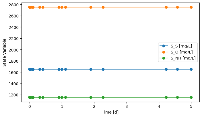
[30]:
# You'll see the mass flows stay constant through the simulation period,
# but still it means the system was simulated dynamically.
fig, ax = MS2.scope.plot_time_series(('S_S', 'S_NH', 'S_O'))
Many commonly used unit operations, such as Pump, Mixer, Splitter, and HydraulicDelay, have implemented the fundamental methods to be used in a dynamic system. You can always refer to the source codes of these units to learn more about how they work.
Back to top
2.4. Making an inactive CompleteMixTank (_compile_ODE)
As you can see above, it’s not very impressive to dynamically simulate a system without any ODEs. So let’s make a simple inactive complete mix tank. Assume the reactor has a fixed liquid volume \(V\), and thus the effluent volumetric flow rate changes instantly with influents. The mass balance of this type of reactor can be described as:
Equations (10) and (11) are the governing ODEs of this unit.
[31]:
class CompleteMixTank(qs.SanUnit):

    _N_outs = 1
    _ins_size_is_fixed = False

    def __init__(self, ID='', ins=None, outs=(), thermo=None,
                 init_with='WasteStream', V=10, **kwargs):
        qs.SanUnit.__init__(self, ID, ins, outs, thermo, init_with, **kwargs)
        self.V = V

    def _run(self):
        out, = self.outs
        out.mix_from(self.ins)

    def set_init_conc(self,**concentrations):
        cmps = self.thermo.chemicals
        C = np.zeros(len(cmps))
        idx = cmps.indices(list(concentrations.keys()))
        C[idx] = list(concentrations.values())
        self._init_concs = C

    def _init_state(self):
        out, = self.outs
        self._state = np.empty(len(cmps)+1)
        self._state[:-1] = self._init_concs      # first n element be the component concentrations of the mixed stream
        self._state[-1] = out.F_vol*24   # last element be the total volumetric flow
        self._dstate = self._state*0.

    def _update_state(self):
        out, = self.outs
        out.state = self._state

    def _update_dstate(self):
        out, = self.outs
        out.dstate = self._dstate

    @property
    def ODE(self):
        if self._ODE is None:
            self._compile_ODE()
        return self._ODE

    def _compile_ODE(self):
        _dstate = self._dstate
        _update_dstate = self._update_dstate
        V = self.V
        def dy_dt(t, y_ins, y, dy_ins):
            Q_ins = y_ins[:,-1]
            C_ins = y_ins[:,:-1]
            dQ_ins = dy_ins[:,-1]
            Q = sum(Q_ins)   # equation (9)
            C = y[:-1]
            _dstate[-1] = sum(dQ_ins) # dQ, equation (10)
            _dstate[:-1] = (Q_ins @ C_ins - Q*C)/V # dC, equation (11)
            _update_dstate()
        self._ODE = dy_dt
Note: 1. All
SanUnit._ODEmust take exactly these four postional arguments:t,y_ins, anddy_insare the same as the ones inSanUnit._AE.yis a 1dnumpy.array, because it is equal to the_statearray of the unit.
Unlike
_AE, allSanUnit._ODEupdates only the_dstatearray of theSanUnit, and only calls_update_dstateafterwards.
[32]:
# Let's see if it works
CMT = CompleteMixTank(ins=(inf1.copy(), inf2.copy()), V=50,
                      isdynamic=True)
dyn_sys3 = qs.System(path=(CMT,))
dyn_sys3.set_dynamic_tracker(CMT)

# To make it more interesting, we'll set the initial condition to be
# something not the steady state.
CMT.set_init_conc(S_S=500, S_NH=700, S_O=290)
dyn_sys3.simulate(t_span=(0,5))
[33]:
CMT.scope.plot_time_series(('S_NH', 'S_S', 'S_O'))
[33]:
(<Figure size 800x450 with 1 Axes>,
 <Axes: xlabel='Time [d]', ylabel='State Variable'>)

Many commonly used unit operations described by ODEs have been implemented in QSDsan, such as CSTR, BatchExperiment, and FlatBottomCircularClarifier.
Back to top
3. Other convenient features
3.1. ExogenousDynamicVariable
The ExogenousDynamicVariable class is created to enable incorporation of exogenous dynamic variables in unit simulations. By “dynamic”, it means the variable value changes over time. By “exogenous”, it means the variable isn’t explicitly dependent on any unit operation or stream. “Ambient temperature” or “sunlight irradiance” is a good example. They are environmental conditions that are often beyond control but have an effect on the operation or performance of the system.
[34]:
# Check out the documentation
from qsdsan.utils import ExogenousDynamicVariable as EDV
# EDV?
There are generally two ways to create an ExogenousDynamicVariable.
Define the variable as a function of time. Let’s say we want to create a variable to represent the changing reaction temperature. Assume the temperature value [K] can be expressed as \(T = 298.15 + 5\cdot \sin(t)\), indicating that the temperatue fluctuacts around \(25^{\circ}C\) by \(\pm 5^{\circ}C\). Then simply,
T = EDV('T', function=lambda t: 298.15+5*np.sin(t))
Provide time-series data to describe the dynamics of the variable. For demonstration purpose, we’ll just make up the data. In practice, this is convenient if you have real data.
t_arr = np.linspace(0, 5)
y_arr = 298.15+5*np.sin(t_arr)
T = EDV('T', t=t_arr, y=y_arr)
For convenience, ExogenousDynamicVariable also has a classmethod that enables batch creation of multiple variables at once. We just need to provide a file of the time-series data, including a column t for time points and additional columns of the variable values. See the documentation of ExogenousDynamicVariable.batch_init for detailed usage.
[35]:
# EDV.batch_init?
Once created, these ExogenousDynamicVariable objects can be incorporated into any SanUnit upon its initialization or through the SanUnit.exo_dynamic_vars property setter.
[36]:
# Let's see an example
from exposan.metab import create_system
sys_mt = create_system()
uf_mt = sys_mt.flowsheet.unit
uf_mt.R1.exo_dynamic_vars
All impact indicators have been removed from the registry.
All impact items have been removed from the registry.
[36]:
(<ExogenousDynamicVariable: T>,)
[37]:
# The evaluation of these variables during unit simulation is done through
# the `eval_exo_dynamic_vars` method
uf_mt.R1.eval_exo_dynamic_vars(t=0.1)
[37]:
[295.15]
Back to top
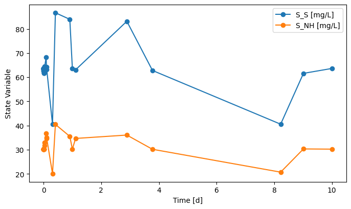
3.2. DynamicInfluent
The DynamicInfluent is a SanUnit subclass for generating dynamic influent streams from user-defined time-series data. The use of this class is, to some extent, similar to an ExogenousDynamicVariable.
[38]:
from qsdsan.sanunits import DynamicInfluent as DI
# DI?
[39]:
qs.set_thermo(bsm1.cmps)
DI1 = DI(outs=('dynamic_stream',))
sys_di = qs.System(path=(DI1,))
sys_di.set_dynamic_tracker(DI1)
sys_di.simulate(t_span=(0, 10))
DI1.scope.plot_time_series(('S_NH', 'S_S'))
[39]:
(<Figure size 800x450 with 1 Axes>,
 <Axes: xlabel='Time [d]', ylabel='State Variable'>)
Back to top