Process Modeling 101
Prepared by:
Covered topics:
1. Introduction
2. System Setup
3. System Simulation
To run tutorials in your browser, go to this Binder page.
[1]:
import qsdsan as qs
print(f'This tutorial was made with qsdsan v{qs.__version__}.')
This tutorial was made with qsdsan v1.2.1.
[2]:
# Import packages
import numpy as np, pandas as pd
from qsdsan import sanunits as su, processes as pc, WasteStream, System
from qsdsan.utils import time_printer, load_data, get_SRT

import warnings
warnings.filterwarnings('ignore')             # to ignore Pandas future warning & NumbaPerformanceWarning
1. Introduction
In this tutorial, we will explore how each QSDsan class is used in practical process simulation.
For this purpose, we will utilize an example system consisting of five-compartment activated sludge reactor followed by a flat-bottom circular clarifier. In addition, as a process model, Activated Sludge Model No. 2d (ASM2d) will be employed.

Back to top
2. System Setup
2.1. Component
Chemicals or biomass existing in a system can be expressed using the Component class of QSDsan.

[3]:
# Components
cmps = pc.create_asm2d_cmps()           # create components of ASM2d
                                        # you don't need to define each component one by one.
                                        # compiled components for ASM2d are already available.

cmps.show()                             # 18 components of ASM2d + water (X_TSS was excluded due to redundancy.)
CompiledComponents([S_O2, S_N2, S_NH4, S_NO3, S_PO4, S_F, S_A, S_I, S_ALK, X_I, X_S, X_H, X_PAO, X_PP, X_PHA, X_AUT, X_MeOH, X_MeP, H2O])
S_O2: Dissolved oxygen, S_N2: Dinitrogen, S_NH4: Ammonium plus ammonia nitrogen, S_NO3: Nitrate plus nitrite nitrogen (NO3-N + NO2-N), S_PO4: Inorganic soluble phosphorus, primarily orthophosphates, S_F: Fermentable, readily biodegradable organic substrates, S_A: Fermentation products, considered to be acetate, S_I: Inert soluble organic material, S_ALK: Alkalinity of the wastewater, X_I: Inert particulate organic material, X_S: Slowly biodegradable substrates, X_H: Heterotrophic organisms, X_PAO: Phosphate-accumulating organisms, PAO, X_PP: Poly-phosphate, X_PHA: A cell internal storage product of phosphorus-accumulating organisms, PAO, X_AUT: Nitrifying organisms, X_MeOH: Metal-hydroxides, X_MeP: Metal-phosphate, MePO4
[4]:
cmps.S_A.show(chemical_info=True) # each component stores thermodynamic properties.
Component: S_A (phase_ref='l')
[Names]  CAS: 64-19-7
         InChI: C2H4O2/c1-2(3)4/h1H3...
         InChI_key: QTBSBXVTEAMEQO-U...
         common_name: acetic acid
         iupac_name: ('ethanoic acid...
         pubchemid: 176
         smiles: CC(=O)O
         formula: C2H4O2
[Groups] Dortmund: <1CH3, 1COOH>
         UNIFAC: <1CH3, 1COOH>
         PSRK: <1CH3, 1COOH>
         NIST: <Empty>
[Data]   MW: 60.052 g/mol
         Tm: 289.85 K
         Tb: 391.05 K
         Tt: 289.69 K
         Tc: 590.7 K
         Pt: 1267.7 Pa
         Pc: 5.78e+06 Pa
         Vc: 0.000171 m^3/mol
         Hf: -4.8358e+05 J/mol
         S0: 159.8 J/K/mol
         LHV: 7.87e+05 J/mol
         HHV: 8.7502e+05 J/mol
         Hfus: 11730 J/mol
         Sfus: None
         omega: 0.4218
         dipole: 1.7 Debye
         similarity_variable: 0.13322
         iscyclic_aliphatic: 0
         combustion: {'CO2': 2, 'O2'...
Component-specific properties:
[Others] measured_as: COD
         description: Acetate
         particle_size: Soluble
         degradability: Readily
         organic: True
         i_C: 0.37535 g C/g COD
         i_N: 0 g N/g COD
         i_P: 0 g P/g COD
         i_K: 0 g K/g COD
         i_Mg: 0 g Mg/g COD
         i_Ca: 0 g Ca/g COD
         i_mass: 0.93835 g mass/g COD
         i_charge: -0.015625 mol +/g COD
         i_COD: 1 g COD/g COD
         i_NOD: 0 g NOD/g COD
         f_BOD5_COD: 0.717
         f_uBOD_COD: 0.8628
         f_Vmass_Totmass: 1
         chem_MW: 60.052
2.2. WasteStream
Mass and energy flow within the system can be represented using the WastStream class of QSDsan.

[5]:
# Parameters (flowrates, temperature)
Q_inf = 18446                               # influent flowrate [m3/d]
Q_was = 385                                 # sludge wastage flowrate [m3/d]
Q_ext = 18446                               # external recycle flowrate [m3/d]
                                            # internal recycle flowrate will be defined later using split ratio.
                                            # effluent flowrate will be calculated as the amount remaining after recycling and wastage.

Temp = 273.15+20                            # temperature [K]
[6]:
# Create influent, effluent, recycle stream
influent = WasteStream('influent', T=Temp)                         # create an empty wastestream with specified temperature
effluent = WasteStream('effluent', T=Temp)

int_recycle = WasteStream('internal_recycle', T=Temp)
ext_recycle = WasteStream('external_recycle', T=Temp)
wastage = WasteStream('wastage', T=Temp)                           # streams between the reactors will be
                                                                   # automatically assigned when we define SanUnit.
[7]:
# Set the influent composition
default_inf_kwargs = {                                             # default influent composition
    'concentrations': {                                            # you can set concentration of each component separately.
      'S_I': 14,
      'X_I': 26.5,
      'S_F': 20.1,
      'S_A': 94.3,
      'X_S': 409.75,
      'S_NH4': 31,
      'S_N2': 0,
      'S_NO3': 0.266,
      'S_PO4': 2.8,
      'X_PP': 0.05,
      'X_PHA': 0.5,
      'X_H': 0.15,
      'X_AUT': 0,
      'X_PAO': 0,
      'S_ALK':7*12,
      },
    'units': ('m3/d', 'mg/L'),                                     # ('input total flowrate', 'input concentrations')
    }

influent.set_flow_by_concentration(Q_inf, **default_inf_kwargs)    # set flowrate and composition of empty influent WasteStream
[8]:
influent # wastestream stores bulk properties of the stream, as well as concentration of each component.
WasteStream: influent
 phase: 'l', T: 293.15 K, P: 101325 Pa
 flow (g/hr): S_NH4  2.38e+04
              S_NO3  204
              S_PO4  2.15e+03
              S_F    1.54e+04
              S_A    7.25e+04
              S_I    1.08e+04
              S_ALK  6.46e+04
              X_I    2.04e+04
              X_S    3.15e+05
              X_H    115
              X_PP   38.4
              X_PHA  384
              H2O    7.67e+08
 WasteStream-specific properties:
  pH         : 7.0
  Alkalinity : 2.5 mg/L
  COD        : 565.3 mg/L
  BOD        : 320.1 mg/L
  TC         : 271.4 mg/L
  TOC        : 187.4 mg/L
  TN         : 48.9 mg/L
  TP         : 7.4 mg/L
  TK         : 0.1 mg/L
 Component concentrations (mg/L):
  S_NH4   31.0
  S_NO3   0.3
  S_PO4   2.8
  S_F     20.1
  S_A     94.3
  S_I     14.0
  S_ALK   84.0
  X_I     26.5
  X_S     409.8
  X_H     0.2
  X_PP    0.1
  X_PHA   0.5
  H2O     998426.3
[9]:
influent.get_VSS() # you can also retreive other information, such as VSS, TSS, TDS, etc.
[9]:
324.9843750592503
2.3. Process
Chemical or biological reactions occurring within the system can be included using the Process class of QSDsan.
2.3.1. Aeration

[10]:
# Parameters (volumes)
V_an = 1000                                 # anoxic zone tank volume [m3/d]
V_ae = 1333                                 # aerated zone tank volume [m3/d]
[11]:
# Aeration model
aer1 = pc.DiffusedAeration('aer1', DO_ID='S_O2', KLa=240, DOsat=8.0, V=V_ae)             # aeration model for Tank 3 & Tank 4
aer2 = pc.DiffusedAeration('aer2', DO_ID='S_O2', KLa=84, DOsat=8.0, V=V_ae)              # aeration model for Tank 5
DO_ID: The component ID of dissolved oxygen (DO). KLa: Oxygen mass transfer coefficient. DOsat: Surface DO saturation concentration. V: Reactor volume
[12]:
aer1
Process: aer1
[stoichiometry]      S_O2: 1
[reference]          S_O2
[rate equation]      KLa*(DOsat - S_O2)
[parameters]         KLa: 240
                     DOsat: 8
[dynamic parameters]
2.3.2. ASM2d

[13]:
# ASM2d
asm2d = pc.ASM2d()                       # create ASM2d processes
asm2d.show()                             # 21 processes in ASM2d
ASM2d([aero_hydrolysis, anox_hydrolysis, anae_hydrolysis, hetero_growth_S_F, hetero_growth_S_A, denitri_S_F, denitri_S_A, ferment, hetero_lysis, PAO_storage_PHA, aero_storage_PP, PAO_aero_growth_PHA, PAO_lysis, PP_lysis, PHA_lysis, auto_aero_growth, auto_lysis, precipitation, redissolution, anox_storage_PP, PAO_anox_growth])
[14]:
asm2d.aero_hydrolysis # Each process includes stoichiometry, rate equation, and parameters.
Process: aero_hydrolysis
[stoichiometry]      S_NH4: 0.02*f_SI + 0.01
                     S_PO4: 0.01*f_SI
                     S_F: 1.0 - 1.0*f_SI
                     S_I: 1.0*f_SI
                     S_ALK: 0.0113*f_SI + 0.00858
                     X_S: -1.00
[reference]          X_S
[rate equation]      K_h*S_O2*X_S/((K_O2 + S_O2)*...
[parameters]         f_SI: 0
                     Y_H: 0.625
                     f_XI_H: 0.1
                     Y_PAO: 0.625
                     Y_PO4: 0.4
                     Y_PHA: 0.2
                     f_XI_PAO: 0.1
                     Y_A: 0.24
                     f_XI_AUT: 0.1
                     K_h: 3
                     eta_NO3: 0.6
                     eta_fe: 0.4
                     K_O2: 0.2
                     K_NO3: 0.5
                     K_X: 0.1
                     mu_H: 6
                     q_fe: 3
                     eta_NO3_H: 0.8
                     b_H: 0.4
                     K_O2_H: 0.2
                     K_F: 4
                     K_fe: 4
                     K_A_H: 4
                     K_NO3_H: 0.5
                     K_NH4_H: 0.05
                     K_P_H: 0.01
                     K_ALK_H: 1.2
                     q_PHA: 3
                     q_PP: 1.5
                     mu_PAO: 1
                     eta_NO3_PAO: 0.6
                     b_PAO: 0.2
                     b_PP: 0.2
                     b_PHA: 0.2
                     K_O2_PAO: 0.2
                     K_NO3_PAO: 0.5
                     K_A_PAO: 4
                     K_NH4_PAO: 0.05
                     K_PS: 0.2
                      K_P_PAO: K_P_PAO
                     K_ALK_PAO: 1.2
                     K_PP: 0.01
                     K_MAX: 0.34
                     K_IPP: 0.02
                     K_PHA: 0.01
                     mu_AUT: 1
                     b_AUT: 0.15
                     K_O2_AUT: 0.5
                     K_NH4_AUT: 1
                     K_ALK_AUT: 6
                     K_P_AUT: 0.01
                     k_PRE: 1
                     k_RED: 0.6
                     K_ALK_PRE: 6
                     K_P_PAO: 0.01
[dynamic parameters]
[15]:
# Petersen stoichiometric matrix of ASM2d
pd.set_option('display.max_columns', None)                  # to display all columns

asm2d.stoichiometry
[15]:
| S_O2 | S_N2 | S_NH4 | S_NO3 | S_PO4 | S_F | S_A | S_I | S_ALK | X_I | X_S | X_H | X_PAO | X_PP | X_PHA | X_AUT | X_MeOH | X_MeP | H2O | |
|---|---|---|---|---|---|---|---|---|---|---|---|---|---|---|---|---|---|---|---|
| aero_hydrolysis | 0 | 0 | 0.01 | 0 | 0 | 1 | 0 | 0 | 0.00858 | 0 | -1 | 0 | 0 | 0 | 0 | 0 | 0 | 0 | 0 |
| anox_hydrolysis | 0 | 0 | 0.01 | 0 | 0 | 1 | 0 | 0 | 0.00858 | 0 | -1 | 0 | 0 | 0 | 0 | 0 | 0 | 0 | 0 |
| anae_hydrolysis | 0 | 0 | 0.01 | 0 | 0 | 1 | 0 | 0 | 0.00858 | 0 | -1 | 0 | 0 | 0 | 0 | 0 | 0 | 0 | 0 |
| hetero_growth_S_F | -0.6 | 0 | -0.022 | 0 | -0.004 | -1.6 | 0 | 0 | -0.0165 | 0 | 0 | 1 | 0 | 0 | 0 | 0 | 0 | 0 | 0 |
| hetero_growth_S_A | -0.6 | 0 | -0.07 | 0 | -0.02 | 0 | -1.6 | 0 | 0.252 | 0 | 0 | 1 | 0 | 0 | 0 | 0 | 0 | 0 | 0 |
| denitri_S_F | 0 | 0.21 | -0.022 | -0.21 | -0.004 | -1.6 | 0 | 0 | 0.164 | 0 | 0 | 1 | 0 | 0 | 0 | 0 | 0 | 0 | 0 |
| denitri_S_A | 0 | 0.21 | -0.07 | -0.21 | -0.02 | 0 | -1.6 | 0 | 0.432 | 0 | 0 | 1 | 0 | 0 | 0 | 0 | 0 | 0 | 0 |
| ferment | 0 | 0 | 0.03 | 0 | 0.01 | -1 | 1 | 0 | -0.168 | 0 | 0 | 0 | 0 | 0 | 0 | 0 | 0 | 0 | 0 |
| hetero_lysis | 0 | 0 | 0.032 | 0 | 0.01 | 0 | 0 | 0 | 0.0216 | 0.1 | 0.9 | -1 | 0 | 0 | 0 | 0 | 0 | 0 | 0 |
| PAO_storage_PHA | 0 | 0 | 0 | 0 | 0.4 | 0 | -1 | 0 | 0.11 | 0 | 0 | 0 | 0 | -0.4 | 1 | 0 | 0 | 0 | 0 |
| aero_storage_PP | -0.2 | 0 | 0 | 0 | -1 | 0 | 0 | 0 | 0.194 | 0 | 0 | 0 | 0 | 1 | -0.2 | 0 | 0 | 0 | 0 |
| PAO_aero_growth_PHA | -0.6 | 0 | -0.07 | 0 | -0.02 | 0 | 0 | 0 | -0.0484 | 0 | 0 | 0 | 1 | 0 | -1.6 | 0 | 0 | 0 | 0 |
| PAO_lysis | 0 | 0 | 0.032 | 0 | 0.01 | 0 | 0 | 0 | 0.0216 | 0.1 | 0.9 | 0 | -1 | 0 | 0 | 0 | 0 | 0 | 0 |
| PP_lysis | 0 | 0 | 0 | 0 | 1 | 0 | 0 | 0 | -0.194 | 0 | 0 | 0 | 0 | -1 | 0 | 0 | 0 | 0 | 0 |
| PHA_lysis | 0 | 0 | 0 | 0 | 0 | 0 | 1 | 0 | -0.188 | 0 | 0 | 0 | 0 | 0 | -1 | 0 | 0 | 0 | 0 |
| auto_aero_growth | -18 | 0 | -4.24 | 4.17 | -0.02 | 0 | 0 | 0 | -7.2 | 0 | 0 | 0 | 0 | 0 | 0 | 1 | 0 | 0 | 0 |
| auto_lysis | 0 | 0 | 0.032 | 0 | 0.01 | 0 | 0 | 0 | 0.0216 | 0.1 | 0.9 | 0 | 0 | 0 | 0 | -1 | 0 | 0 | 0 |
| precipitation | 0 | 0 | 0 | 0 | -1 | 0 | 0 | 0 | 0.582 | 0 | 0 | 0 | 0 | 0 | 0 | 0 | -3.45 | 4.87 | 0 |
| redissolution | 0 | 0 | 0 | 0 | 1 | 0 | 0 | 0 | -0.582 | 0 | 0 | 0 | 0 | 0 | 0 | 0 | 3.45 | -4.87 | 0 |
| anox_storage_PP | 0 | 0.07 | 0 | -0.07 | -1 | 0 | 0 | 0 | 0.254 | 0 | 0 | 0 | 0 | 1 | -0.2 | 0 | 0 | 0 | 0 |
| PAO_anox_growth | 0 | 0.208 | -0.0683 | -0.21 | -0.02 | 0 | 0 | 0 | 0.133 | 0 | 0 | 0 | 1 | 0 | -1.6 | 0 | 0 | 0 | 0 |
[16]:
# Rate equations of ASM2d
asm2d.rate_equations
[16]:
| rate_equation | |
|---|---|
| aero_hydrolysis | 3.0*S_O2*X_S/((0.1 + X_S/X_H)*(... |
| anox_hydrolysis | 0.36*S_NO3*X_S/((0.1 + X_S/X_H)... |
| anae_hydrolysis | 0.12*X_S/((0.1 + X_S/X_H)*(S_NO... |
| hetero_growth_S_F | 6.0*S_ALK*S_F**2*S_NH4*S_O2*S_P... |
| hetero_growth_S_A | 6.0*S_A**2*S_ALK*S_NH4*S_O2*S_P... |
| denitri_S_F | 0.96*S_ALK*S_F**2*S_NH4*S_NO3*S... |
| denitri_S_A | 0.96*S_A**2*S_ALK*S_NH4*S_NO3*S... |
| ferment | 0.3*S_ALK*S_F*X_H/((S_ALK + 1.2... |
| hetero_lysis | 0.4*X_H |
| PAO_storage_PHA | 3.0*S_A*S_ALK*X_PP/((0.01 + X_P... |
| aero_storage_PP | 1.5*S_ALK*S_O2*S_PO4*X_PHA*(0.3... |
| PAO_aero_growth_PHA | 1.0*S_ALK*S_NH4*S_O2*S_PO4*X_PH... |
| PAO_lysis | 0.2*S_ALK*X_PAO/(S_ALK + 1.2) |
| PP_lysis | 0.2*S_ALK*X_PP/(S_ALK + 1.2) |
| PHA_lysis | 0.2*S_ALK*X_PHA/(S_ALK + 1.2) |
| auto_aero_growth | 1.0*S_ALK*S_NH4*S_O2*S_PO4*X_AU... |
| auto_lysis | 0.15*X_AUT |
| precipitation | 1.0*S_PO4*X_MeOH |
| redissolution | 0.6*S_ALK*X_MeP/(S_ALK + 6.0) |
| anox_storage_PP | 0.18*S_ALK*S_NO3*S_PO4*X_PHA*(0... |
| PAO_anox_growth | 0.12*S_ALK*S_NH4*S_NO3*S_PO4*X_... |
2.4. SanUnit
Reactors constituting the system can be represented using the SanUnit class of QSDsan.

[17]:
# Anoxic reactors (Tank 1 & Tank 2)
A1 = su.CSTR('A1', ins=[influent, int_recycle, ext_recycle], V_max=V_an,      # As CSTR, 3 input streams, tank volume as V_an
             aeration=None, suspended_growth_model=asm2d)                     # No aeration, biokinetic model as asm2d

A2 = su.CSTR('A2', ins=A1-0, V_max=V_an,                 # ins=A1-0: set influent of A2 as effluent of A1 reactor (to connect A1 with A2)
             aeration=None, suspended_growth_model=asm2d)
ins: Influents to the reactor. outs: Treated effluent from the reactor. V_max: Designed volume, in [m^3]. The default is 1000. aeration: Aeration setting. Either specify a targeted dissolved oxygen concentration in [mg O2/L] or provide a :class:Process object to represent aeration, or None for no aeration. The default is 2.0. suspended_growth_model: The suspended growth biokinetic model. The default is None.
[18]:
A1 # Before simulation, outs are empty.

CSTR: A1
ins...
[0] influent
    phase: 'l', T: 293.15 K, P: 101325 Pa
    flow (g/hr): S_NH4  2.38e+04
                 S_NO3  204
                 S_PO4  2.15e+03
                 S_F    1.54e+04
                 S_A    7.25e+04
                 S_I    1.08e+04
                 S_ALK  6.46e+04
                 X_I    2.04e+04
                 X_S    3.15e+05
                 X_H    115
                 X_PP   38.4
                 X_PHA  384
                 H2O    7.67e+08
    WasteStream-specific properties:
     pH         : 7.0
     COD        : 565.3 mg/L
     BOD        : 320.1 mg/L
     TC         : 271.4 mg/L
     TOC        : 187.4 mg/L
     TN         : 48.9 mg/L
     TP         : 7.4 mg/L
     TK         : 0.1 mg/L
[1] internal_recycle
    phase: 'l', T: 293.15 K, P: 101325 Pa
    flow: 0
    WasteStream-specific properties: None for empty waste streams
[2] external_recycle
    phase: 'l', T: 293.15 K, P: 101325 Pa
    flow: 0
    WasteStream-specific properties: None for empty waste streams
outs...
[0] ws1  to  CSTR-A2
    phase: 'l', T: 298.15 K, P: 101325 Pa
    flow: 0
    WasteStream-specific properties: None for empty waste streams
[19]:
# Aerated reactors (Tank 3, Tank 4, Tank 5)
O1 = su.CSTR('O1', ins=A2-0, V_max=V_ae, aeration=aer1,                          # tank volume as V_ae with aeration model1
             DO_ID='S_O2', suspended_growth_model=asm2d)

O2 = su.CSTR('O2', ins=O1-0, V_max=V_ae, aeration=aer1,
             DO_ID='S_O2', suspended_growth_model=asm2d)

O3 = su.CSTR('O3', ins=O2-0, outs=[int_recycle, 'treated'], split=[0.6, 0.4],    # 60% of efflunet to internal recycle, 40% to clarifier
             V_max=V_ae, aeration=aer2,
             DO_ID='S_O2', suspended_growth_model=asm2d)
[20]:
O3

CSTR: O3
ins...
[0] ws7  from  CSTR-O2
    phase: 'l', T: 298.15 K, P: 101325 Pa
    flow: 0
    WasteStream-specific properties: None for empty waste streams
outs...
[0] internal_recycle  to  CSTR-A1
    phase: 'l', T: 293.15 K, P: 101325 Pa
    flow: 0
    WasteStream-specific properties: None for empty waste streams
[1] treated
    phase: 'l', T: 298.15 K, P: 101325 Pa
    flow: 0
    WasteStream-specific properties: None for empty waste streams
[21]:
# Clarifier
C1 = su.FlatBottomCircularClarifier('C1', ins=O3-1, outs=[effluent, ext_recycle, wastage],  # O3-1: second effluent of O3, three outs
                                    underflow=Q_ext, wastage=Q_was, surface_area=1500,
                                    height=4, N_layer=10, feed_layer=5,                     # modeled as a 10 layer non-reactive unit
                                    X_threshold=3000, v_max=474, v_max_practical=250,
                                    rh=5.76e-4, rp=2.86e-3, fns=2.28e-3)
underflow: Designed recycling sludge flowrate (RAS), in [m^3/d]. The default is 2000. wastage: Designed wasted sludge flowrate (WAS), in [m^3/d]. The default is 385. surface_area: Surface area of the clarifier, in [m^2]. The default is 1500. height: Height of the clarifier, in [m]. The default is 4. N_layer: The number of layers to model settling. The default is 10. feed_layer: The feed layer counting from top to bottom. The default is 4. X_threshold: Threshold suspended solid concentration, in [g/m^3]. The default is 3000. v_max: Maximum theoretical (i.e. Vesilind) settling velocity, in [m/d]. The default is 474. v_max_practical: Maximum practical settling velocity, in [m/d]. The default is 250. rh: Hindered zone settling parameter in the double-exponential settling velocity function, in [m^3/g]. The default is 5.76e-4. rp: Flocculant zone settling parameter in the double-exponential settling velocity function, in [m^3/g]. The default is 2.86e-3. fns: Non-settleable fraction of the suspended solids, dimensionless. Must be within [0, 1]. The default is 2.28e-3.
2.5. System
System objects are used to organize unit operations in a certain order and facilitate mass and energy convergence, techno-economic analysis (TEA), and life cycle assessment (LCA).

2.5.1. Create system
[22]:
# Create system
sys = System('example_system', path=(A1, A2, O1, O2, O3, C1), recycle=(int_recycle, ext_recycle))     # path: the order of reactor
[23]:
# System diagram
sys.diagram()

[24]:
sys # before running the simulation, 'outs' have nothing

System: example_system
ins...
[0] influent
    phase: 'l', T: 293.15 K, P: 101325 Pa
    flow (kmol/hr): S_NH4  1.4
                    S_NO3  0.0033
                    S_PO4  0.0112
                    S_F    15.4
                    S_A    1.21
                    S_I    10.8
                    S_ALK  1.06
                    ...    4.29e+04
outs...
[0] effluent
    phase: 'l', T: 293.15 K, P: 101325 Pa
    flow: 0
[1] wastage
    phase: 'l', T: 293.15 K, P: 101325 Pa
    flow: 0
2.5.2. Set initial conditions of reactors
[25]:
# Import initial condition excel file
df = load_data('assets/tutorial_13/initial_conditions_asm2d.xlsx', sheet='default')
[26]:
df # Unlike other reactors, C1 has 3 rows for each of soluble, solids, and tss.
[26]:
| S_O2 | S_NH4 | S_NO3 | S_PO4 | S_F | S_A | S_I | S_ALK | X_I | X_S | X_H | X_PAO | X_PP | X_PHA | X_AUT | |
|---|---|---|---|---|---|---|---|---|---|---|---|---|---|---|---|
| A1 | 0.00213 | 7.23 | 10.2 | 4.45 | 0.211 | 0.0265 | 15.9 | 67 | 2.28e+03 | 84.4 | 3.78e+03 | 322 | 37.2 | 0.0517 | 218 |
| A2 | 0.001 | 22.4 | 2.4 | 4.24 | 6.68 | 53.8 | 14.5 | 79 | 0 | 84.1 | 207 | 18.2 | 4.25 | 3.59 | 11.9 |
| O2 | 2 | 16.5 | 4.31 | 5.48 | 1.9 | 2.73 | 13.7 | 82.6 | 611 | 77.3 | 1.04e+03 | 86.4 | 6.45 | 11 | 58 |
| O3 | 2 | 10.9 | 9.31 | 2.62 | 0.649 | 0.163 | 14.1 | 74.2 | 662 | 59.3 | 1.14e+03 | 95.7 | 9.99 | 7.24 | 64 |
| O1 | 2 | 0.111 | 26.1 | 2.32 | 0.276 | 0.00407 | 18.2 | 46.1 | 2.24e+03 | 61.1 | 3.79e+03 | 322 | 38.4 | 0.00852 | 218 |
| C1_s | 2 | 0.114 | 20.9 | 0.356 | 0.307 | 0.00537 | 20.1 | 49.6 | NaN | NaN | NaN | NaN | NaN | NaN | NaN |
| C1_x | NaN | NaN | NaN | NaN | NaN | NaN | NaN | NaN | 2.24e+03 | 61.1 | 3.79e+03 | 322 | 38.4 | 0.00852 | 218 |
| C1_tss | 17.8 | 27.9 | 44.9 | 90.5 | 305 | 304 | 306 | 304 | 304 | 5.83e+03 | NaN | NaN | NaN | NaN | NaN |
[27]:
# Create a function to set initial conditions of the reactors
def batch_init(sys, df):
    dct = df.to_dict('index')                                         # convert the DataFrame to a dictionary.
    u = sys.flowsheet.unit                                            # unit registry (A1, A2, O1, O2, O3, C1)

    for k in [u.A1, u.A2, u.O1, u.O2, u.O3]:                          # for A1, A2, O1, O2, O3 reactor,
        k.set_init_conc(**dct[k._ID])                                 # A1.set_init_conc(**dct[k_ID])

    c1s = {k:v for k,v in dct['C1_s'].items() if v>0}                # for clarifier, need to use different methods
    c1x = {k:v for k,v in dct['C1_x'].items() if v>0}
    tss = [v for v in dct['C1_tss'].values() if v>0]
    u.C1.set_init_solubles(**c1s)                                     # set solubles
    u.C1.set_init_sludge_solids(**c1x)                                # set sludge solids
    u.C1.set_init_TSS(tss)                                            # set TSS
[28]:
batch_init(sys, df)
Back to top
3. System Simulation
3.1. Run simulation
[29]:
# Simulation settings
sys.set_dynamic_tracker(influent, effluent, A1, A2, O1, O2, O3, C1, wastage)           # what you want to track changes in concentration
sys.set_tolerance(rmol=1e-6)

biomass_IDs = ('X_H', 'X_PAO', 'X_AUT')
[30]:
# Simulation settings
t = 50                          # total time for simulation
t_step = 1                      # times at which to store the computed solution

method = 'BDF'                  # integration method to use
# method = 'RK45'
# method = 'RK23'
# method = 'DOP853'
# method = 'Radau'
# method = 'LSODA'

# https://docs.scipy.org/doc/scipy/reference/generated/scipy.integrate.solve_ivp.html
[31]:
# Run simulation, this could take several minuates
sys.simulate(state_reset_hook='reset_cache',
             t_span=(0,t),
             t_eval=np.arange(0, t+t_step, t_step),
             method=method,
            # export_state_to=f'sol_{t}d_{method}.xlsx',               # uncomment to export simulation result as excel file
            )
[32]:
srt = get_SRT(sys, biomass_IDs)
print(f'Estimated SRT assuming at steady state is {round(srt, 2)} days')
Estimated SRT assuming at steady state is 10.02 days
[33]:
sys # now you have 'outs' info.

System: example_system
Highest convergence error among components in recycle
streams {C1-1, O3-0} after 5 loops:
- flow rate   1.17e-06 kmol/hr (9.1e-10%)
- temperature 2.63e-08 K (9e-09%)
ins...
[0] influent
    phase: 'l', T: 293.15 K, P: 101325 Pa
    flow (kmol/hr): S_NH4  1.4
                    S_NO3  0.0033
                    S_PO4  0.0112
                    S_F    15.4
                    S_A    1.21
                    S_I    10.8
                    S_ALK  1.06
                    ...    4.29e+04
outs...
[0] effluent
    phase: 'l', T: 293.15 K, P: 101325 Pa
    flow (kmol/hr): S_O2   0.000506
                    S_N2   0.00716
                    S_NH4  1.64
                    S_NO3  2.21e-09
                    S_PO4  0.015
                    S_F    0.973
                    S_A    0.111
                    ...    4.17e+04
[1] wastage
    phase: 'l', T: 293.15 K, P: 101325 Pa
    flow (kmol/hr): S_O2   1.08e-05
                    S_N2   0.000153
                    S_NH4  0.0349
                    S_NO3  4.72e-11
                    S_PO4  0.000321
                    S_F    0.0207
                    S_A    0.00237
                    ...    1.04e+03
3.2. Check simulation results
[34]:
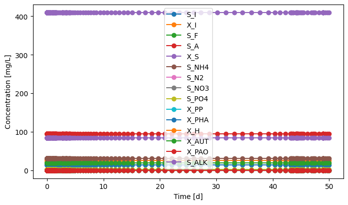
# Influent
influent.scope.plot_time_series(('S_I','X_I','S_F','S_A','X_S','S_NH4','S_N2','S_NO3','S_PO4','X_PP','X_PHA',
                                 'X_H','X_AUT','X_PAO','S_ALK'))      # you can plot how each state variable changes over time

#default_inf_kwargs = {
#    'concentrations': {
#      'S_I': 14,
#      'X_I': 26.5,
#      'S_F': 20.1,
#      'S_A': 94.3,
#      'X_S': 409.75,
#      'S_NH4': 31,
#      'S_N2': 0,
#      'S_NO3': 0.266,
#      'S_PO4': 2.8,
#      'X_PP': 0.05,
#      'X_PHA': 0.5,
#      'X_H': 0.15,
#      'X_AUT': 0,
#      'X_PAO': 0,
#      'S_ALK':7*12,
#      },
#    'units': ('m3/d', 'mg/L'),
#    }                                                               # constant influent setting
[34]:
(<Figure size 800x450 with 1 Axes>,
 <AxesSubplot:xlabel='Time [d]', ylabel='Concentration [mg/L]'>)
[35]:
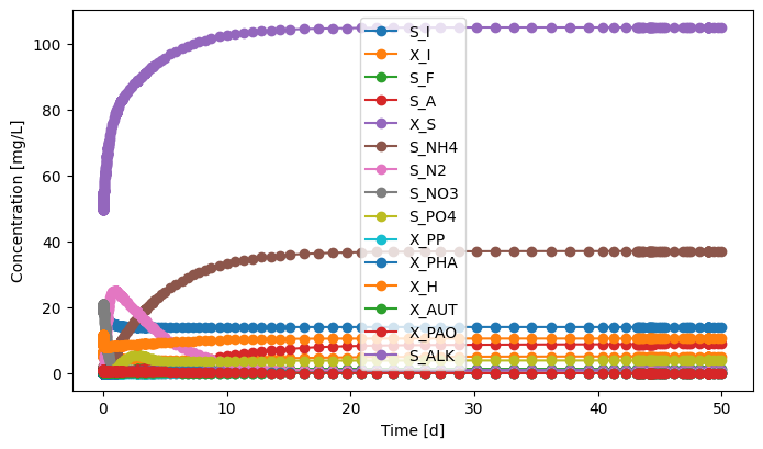
# Effluent
effluent.scope.plot_time_series((('S_I','X_I','S_F','S_A','X_S','S_NH4','S_N2','S_NO3','S_PO4','X_PP','X_PHA',
                                 'X_H','X_AUT','X_PAO','S_ALK')))                   # you can plot how each state variable changes over time
[35]:
(<Figure size 800x450 with 1 Axes>,
 <AxesSubplot:xlabel='Time [d]', ylabel='Concentration [mg/L]'>)
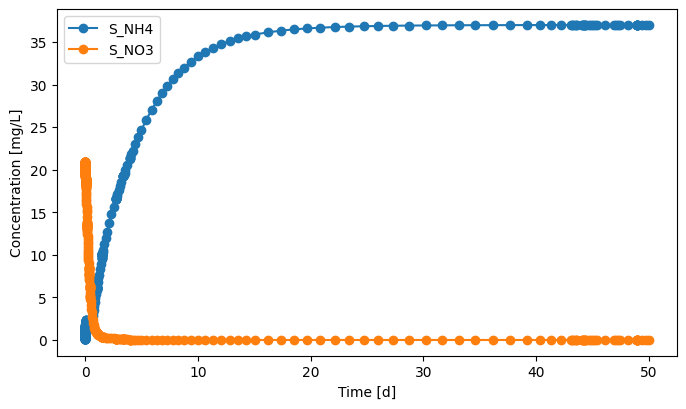
[36]:
effluent.scope.plot_time_series(('S_NH4', 'S_NO3')) # you can plot how each state variable changes over time
[36]:
(<Figure size 800x450 with 1 Axes>,
 <AxesSubplot:xlabel='Time [d]', ylabel='Concentration [mg/L]'>)
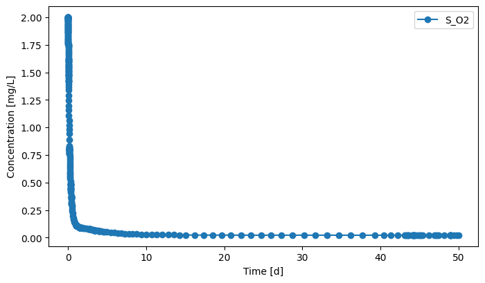
[37]:
effluent.scope.plot_time_series(('S_O2')) # you can plot how each state variable changes over time
[37]:
(<Figure size 800x450 with 1 Axes>,
 <AxesSubplot:xlabel='Time [d]', ylabel='Concentration [mg/L]'>)
Back to top