Anaerobic Digestion Model No. 1 (ADM1)

Click the badge below to try this tutorial interactively in your browser:

You can also run this tutorial inGoogle Colab. It takes a one-time setup per session: follow theColab instructions.

• Prepared by:

  • Ga-Yeong Kim

• Learning objectives. After this tutorial, you will be able to:

  • Apply the ADM1 biokinetic model to anaerobic digestion

  • Set up a multi-component dynamic system

  • Analyze how operating conditions drive the digester response

• Prerequisites: 11. Dynamic Simulation

• Covered topics:

  • 1. Introduction

  • 2. System setup

  • 3. Result discussion

Setup

Import QSDsan and confirm the installed version. An ADM1 example system is also packaged ready-to-run in the adm module of EXPOsan; this notebook builds an equivalent system from scratch so each piece is visible.

import qsdsan as qs
print(f'This tutorial was made with qsdsan v{qs.__version__}')

This tutorial was made with qsdsan v1.5.3

1. Introduction

In Tutorials 10 and 11, we have learned about the foundamentals of process modeling. As a practical example, this tutorial uses ADM1, the International Water Association (IWA)-validated benchmark for anaerobic digestion, as a substantial worked example that uses both at once.

• Tutorial 10 covered how a kinetic model is represented in QSDsan: the Process and Processes classes that hold stoichiometry and rate equations, and the Petersen matrix that tabulates a whole process model. In this tutorial, we will use ADM1, which is a pre-constructed and ready-to-use CompiledProcesses object for ADM1 in QSDsan.

• Tutorial 11 covered how a dynamic simulation is set up and run: the AnaerobicCSTR / CompleteMixTank family of dynamic units, the _state / _dstate methods, the integrator loop, and set_dynamic_tracker for following state evolution. In this tutorial, we will use AnaerobicCSTR, a dynamic SanUnit. We will also construct a dynamic System that contains AnaerobicCSTR for simulation.

1.1. What ADM1 models

ADM1 describes the biochemical and physico-chemical processes for anaerobic digestion (AD).

The biochemical steps are organized as a cascade:

• Disintegration of homogeneous particulates (X_c) into carbohydrates, proteins, and lipids.

• Hydrolysis of those particulates to sugars (S_su), amino acids (S_aa), and long-chain fatty acids (LCFA, S_fa).

• Acidogenesis of sugars and amino acids to volatile fatty acids (VFAs), acetate, and hydrogen.

• Acetogenesis of LCFA and the longer VFAs (valerate, butyrate, propionate) to acetate and hydrogen.

• Methanogenesis in two parallel paths: acetoclastic (S_ac → S_ch4) and hydrogenotrophic (S_h2 → S_ch4).

Seven biomass groups catalyse these steps and decay back into the composite pool.

The physico-chemical equations cover acid/base equilibria (which set the pH) and gas-liquid transfer for H₂, CH₄, and CO₂.

The four canonical AD steps as represented in ADM1. Each band corresponds to one step; the biomass group labelled on each arrow catalyses that conversion.

Reference: Batstone, D. J., et al. (2002). The IWA Anaerobic Digestion Model No. 1 (ADM1). Water Science and Technology, 45(10), 65–73. https://doi.org/10.2166/wst.2002.0292

1.2. Differential-algebraic structure

Implemented as a differential-algebraic (DAE) set, ADM1 has 26 dynamic state variables in the liquid phase and 8 implicit algebraic variables in the headspace (the partial pressures of H₂, CH₄, CO₂, and H₂O, plus the ion balance that sets pH). Implemented as pure ODEs, there are 32 dynamic variables. The figure below shows the DAE shape that AnaerobicCSTR evaluates at each integrator step.

Each integrator step evaluates the liquid-phase ODE block, the headspace algebraic block, and the gas-liquid transfer terms (``k_L·a · (S_aq − K_H · p)``) that link them. Liquid effluent and biogas leave through outflow arrows; the biomass-decay loop (not drawn here) returns active biomass to ``X_c`` in the ODE block.

Note on ``algebraic_h2``. Hydrogen has very fast dynamics relative to the rest of the model (small pool, rapid turnover), which makes the ODE block stiff. AnaerobicCSTR exposes an algebraic_h2 switch: with algebraic_h2=True the S_h2 equation is moved into the algebraic block, removing this source of stiffness at the cost of one extra algebraic equation. The default algebraic_h2=False keeps S_h2 as an ODE, which is what we use throughout this tutorial.

Note: You can find validation of the ADM1 system in EXPOsan.

# Import packages
import numpy as np
from chemicals.elements import molecular_weight as get_mw
from qsdsan import unit_operations as su, process_models as pc, WasteStream, System
from qsdsan.utils import time_printer

1.3. State variables of ADM1

Components were introduced in Tutorial 2; pc.create_adm1_cmps assembles the ADM1-specific set in one call so we don’t have to define each of the 27 components by hand.

# Components
cmps = pc.create_adm1_cmps()           # create state variables for ADM1
cmps.show()                            # 26 components in ADM1 + water

CompiledComponents([
    S_su,  S_aa,  S_fa, S_va,
    S_bu,  S_pro, S_ac, S_h2,
    S_ch4, S_IC,  S_IN, S_I,
    X_c,   X_ch,  X_pr, X_li,
    X_su,  X_aa,  X_fa, X_c4,
    X_pro, X_ac,  X_h2, X_I,
    S_cat, S_an,  H2O,
])

The 26 ADM1 state variables (plus water, which is always present):

• S_su: monosaccharides

• S_aa: amino acids

• S_fa: long-chain fatty acids (LCFA)

• S_va: valerate

• S_bu: butyrate

• S_pro: propionate

• S_ac: acetate

• S_h2: dissolved hydrogen

• S_ch4: dissolved methane

• S_IC: inorganic carbon (dissolved CO₂ and HCO₃⁻)

• S_IN: inorganic nitrogen

• S_I: soluble inerts

• X_c: composites

• X_ch: carbohydrates

• X_pr: proteins

• X_li: lipids

• X_su: biomass that takes up sugars

• X_aa: biomass that takes up amino acids

• X_fa: biomass that takes up LCFA

• X_c4: biomass that takes up C4 fatty acids (valerate and butyrate)

• X_pro: biomass that takes up propionate

• X_ac: biomass that takes up acetate

• X_h2: biomass that takes up hydrogen

• X_I: particulate inerts

• S_cat: other cations

• S_an: other anions

1.4. The ADM1 Process

As covered in Tutorial 10, Processes.load_from_file lets you build a process model from a spreadsheet. pc.ADM1() is the prebuilt variant: the same CompiledProcesses class, with the IWA-specified rate equations and parameters already assembled.

# Processes
adm1 = pc.ADM1()                       # create ADM1 processes
adm1.show()                            # 22 processes in ADM1

ADM1([disintegration, hydrolysis_carbs, hydrolysis_proteins, hydrolysis_lipids, uptake_sugars, uptake_amino_acids, uptake_LCFA, uptake_valerate, uptake_butyrate, uptake_propionate, uptake_acetate, uptake_h2, decay_Xsu, decay_Xaa, decay_Xfa, decay_Xc4, decay_Xpro, decay_Xac, decay_Xh2, h2_transfer, ch4_transfer, IC_transfer])

1.5. Petersen matrix of ADM1

As introduced in Tutorial 10, the table below is the Petersen matrix of ADM1: 22 rows (processes) by 27 columns (components plus water). Each cell is a stoichiometric coefficient.

# Petersen stoichiometric matrix
adm1.stoichiometry

	S_su	S_aa	S_fa	S_va	S_bu	...	X_h2	X_I	S_cat	S_an	H2O
disintegration	0	0	0	0	0	...	0	0.2	0	0	0
hydrolysis_carbs	1	0	0	0	0	...	0	0	0	0	0
hydrolysis_proteins	0	1	0	0	0	...	0	0	0	0	0
hydrolysis_lipids	0.05	0	0.95	0	0	...	0	0	0	0	0
uptake_sugars	-1	0	0	0	0.117	...	0	0	0	0	0
uptake_amino_acids	0	-1	0	0.212	0.239	...	0	0	0	0	0
uptake_LCFA	0	0	-1	0	0	...	0	0	0	0	0
uptake_valerate	0	0	0	-1	0	...	0	0	0	0	0
uptake_butyrate	0	0	0	0	-1	...	0	0	0	0	0
uptake_propionate	0	0	0	0	0	...	0	0	0	0	0
uptake_acetate	0	0	0	0	0	...	0	0	0	0	0
uptake_h2	0	0	0	0	0	...	0.06	0	0	0	0
decay_Xsu	0	0	0	0	0	...	0	0	0	0	0
decay_Xaa	0	0	0	0	0	...	0	0	0	0	0
decay_Xfa	0	0	0	0	0	...	0	0	0	0	0
decay_Xc4	0	0	0	0	0	...	0	0	0	0	0
decay_Xpro	0	0	0	0	0	...	0	0	0	0	0
decay_Xac	0	0	0	0	0	...	0	0	0	0	0
decay_Xh2	0	0	0	0	0	...	-1	0	0	0	0
h2_transfer	0	0	0	0	0	...	0	0	0	0	0
ch4_transfer	0	0	0	0	0	...	0	0	0	0	0
IC_transfer	0	0	0	0	0	...	0	0	0	0	0

22 rows × 27 columns

The rate of production or consumption for a state variable

\(a_{ij}\): the stoichiometric coefficient of component \(j\) in process \(i\) (i.e., value on the \(i\) th row and \(j\) th column of the stoichiometry matrix) \(\rho_i\): process \(i\)’s reaction rate \(r_j\): the overall production or consumption rate of component \(j\)

\[r_j = \sum_i{a_{ij}\cdot\rho_i}\]

In matrix notation, this calculation can be neatly described as

\[\mathbf{r} = \mathbf{A^T} \mathbf{\rho}\]

where \(\mathbf{A}\) is the stoichiometry matrix and \(\mathbf{\rho}\) is the array of process rates.

2. System setup

2.1. Influent & effluent

For illustrative purposes, let’s assume the following setup for the system.

Temp = 273.15+35                                    # temperature [K]
inf = WasteStream('Influent', T=Temp)               # influent
eff = WasteStream('Effluent', T=Temp)               # effluent
gas = WasteStream('Biogas')                         # gas

# Set influent flowrate and concentration
C_mw = get_mw({'C':1})        # molecular weight of carbon
N_mw = get_mw({'N':1})        # molecular weight of nitrogen

Q = 170                                             # influent flowrate [m3/d]
default_inf_kwargs = {
    'concentrations': {
        'S_su':0.01,
        'S_aa':1e-3,
        'S_fa':1e-3,
        'S_va':1e-3,
        'S_bu':1e-3,
        'S_pro':1e-3,
        'S_ac':1e-3,
        'S_h2':1e-8,
        'S_ch4':1e-5,
        'S_IC':0.04*C_mw,
        'S_IN':0.01*N_mw,
        'S_I':0.02,
        'X_c':2.0,
        'X_ch':5.0,
        'X_pr':20.0,
        'X_li':5.0,
        'X_aa':1e-2,
        'X_fa':1e-2,
        'X_c4':1e-2,
        'X_pro':1e-2,
        'X_ac':1e-2,
        'X_h2':1e-2,
        'X_I':25,
        'S_cat':0.04,
        'S_an':0.02,
        },
    'units': ('m3/d', 'kg/m3'),
    }                                                           # concentration of each state variable in influent

inf.set_flow_by_concentration(Q, **default_inf_kwargs)          # set influent concentration
inf

WasteStream: Influent
phase: 'l', T: 308.15 K, P: 101325 Pa
flow (g/hr): S_su   70.8
             S_aa   7.08
             S_fa   7.08
             S_va   7.08
             S_bu   7.08
             S_pro  7.08
             S_ac   7.08
             S_h2   7.08e-05
             S_ch4  0.0708
             S_IC   3.4e+03
             S_IN   992
             S_I    142
             X_c    1.42e+04
             X_ch   3.54e+04
             X_pr   1.42e+05
             ...    6.99e+06
 WasteStream-specific properties:
  pH         : 7.0
  Alkalinity : 2.5 mmol/L
  COD        : 57096.0 mg/L
  BOD        : 12769.4 mg/L
  TC         : 20581.4 mg/L
  TOC        : 20101.0 mg/L
  TN         : 3681.4 mg/L
  TP         : 489.3 mg/L
  TK         : 9.8 mg/L
  TSS        : 32679.7 mg/L
 Component concentrations (mg/L):
  S_su   10.0
  S_aa   1.0
  S_fa   1.0
  S_va   1.0
  S_bu   1.0
  S_pro  1.0
  S_ac   1.0
  S_h2   0.0
  S_ch4  0.0
  S_IC   480.4
  S_IN   140.1
  S_I    20.0
  X_c    2000.0
  X_ch   5000.0
  X_pr   20000.0
  ...

2.2. Reactor

AnaerobicCSTR is the same kind of dynamic unit as the CompleteMixTank from Tutorial 11; it adds the headspace algebraic block shown above.

The key parameters of AnaerobicCSTR are:

• ins: influent WasteStream to the reactor.

• outs: the biogas and the treated effluent(s).

• model: process model used in the reactor.

• HRT: hydraulic retention time [d].

• V_liq: liquid-phase volume [m^3].

• V_gas: headspace volume [m^3].

• model: the kinetic model (typically ADM1-like).

• T: operating temperature [K].

For the complete signature and all parameters (e.g., headspace_P, retain_cmps, fraction_retain), run ?su.AnaerobicCSTR or see the unit operations API.

# Assume an HRT of 5 days, and the gas volume is 10% of the liquid volume in the reactor
HRT = 5
AD = su.AnaerobicCSTR('AD', ins=inf, outs=(gas, eff), model=adm1, V_liq=Q*HRT, V_gas=Q*HRT*0.1, T=Temp)

# anaerobic CSTR with influent, effluent, and biogas
# before running the simulation, 'outs' have nothing
AD.show()

AnaerobicCSTR: AD
ins...
[0] Influent
phase: 'l', T: 308.15 K, P: 101325 Pa
flow (g/hr): S_su   70.8
                S_aa   7.08
                S_fa   7.08
                S_va   7.08
                S_bu   7.08
                S_pro  7.08
                S_ac   7.08
                S_h2   7.08e-05
                S_ch4  0.0708
                S_IC   3.4e+03
                S_IN   992
                S_I    142
                X_c    1.42e+04
                X_ch   3.54e+04
                X_pr   1.42e+05
                ...    6.99e+06
    WasteStream-specific properties:
     pH         : 7.0
     Alkalinity : 2.5 mmol/L
     COD        : 57096.0 mg/L
     BOD        : 12769.4 mg/L
     TC         : 20581.4 mg/L
     TOC        : 20101.0 mg/L
     TN         : 3681.4 mg/L
     TP         : 489.3 mg/L
     TK         : 9.8 mg/L
     TSS        : 32679.7 mg/L
outs...
[0] Biogas
phase: 'l', T: 298.15 K, P: 101325 Pa
flow: 0
    WasteStream-specific properties: None for empty waste streams
[1] Effluent
phase: 'l', T: 308.15 K, P: 101325 Pa
flow: 0
    WasteStream-specific properties: None for empty waste streams

# Set the initial condition of the reactor,
# the closer the intial condition is to the steady state,
# the faster the simulation will converge.
default_init_conds = {
    'S_su': 0.0124*1e3,
    'S_aa': 0.0055*1e3,
    'S_fa': 0.1074*1e3,
    'S_va': 0.0123*1e3,
    'S_bu': 0.0140*1e3,
    'S_pro': 0.0176*1e3,
    'S_ac': 0.0893*1e3,
    'S_h2': 2.5055e-7*1e3,
    'S_ch4': 0.0555*1e3,
    'S_IC': 0.0951*C_mw*1e3,
    'S_IN': 0.0945*N_mw*1e3,
    'S_I': 0.1309*1e3,
    'X_ch': 0.0205*1e3,
    'X_pr': 0.0842*1e3,
    'X_li': 0.0436*1e3,
    'X_su': 0.3122*1e3,
    'X_aa': 0.9317*1e3,
    'X_fa': 0.3384*1e3,
    'X_c4': 0.3258*1e3,
    'X_pro': 0.1011*1e3,
    'X_ac': 0.6772*1e3,
    'X_h2': 0.2848*1e3,
    'X_I': 17.2162*1e3
    }

AD.set_init_conc(**default_init_conds)

2.3. System

As in Tutorial 11, set_dynamic_tracker decides which objects retain their state-trajectory history. Here we pass the two outlet WasteStreams (eff and gas), so eff.scope and gas.scope are populated after the simulation, which is what §3 will plot.

# We need to include the reactor in a system to run the dynamic simulation,
# and we need to tell the system what we want to track.
sys = System('Anaerobic_Digestion', path=(AD,))                 # aggregation of unit operations
sys.set_dynamic_tracker(eff, gas)                               # what you want to track changes in concentration
sys.show()                                                      # before running the simulation, 'outs' have nothing

System: Anaerobic_Digestion
ins...
[0] Influent
    phase: 'l', T: 308.15 K, P: 101325 Pa
    flow (kmol/hr): S_su   0.000369
                    S_aa   0.00708
                    S_fa   9.62e-06
                    S_va   3.41e-05
                    S_bu   4.43e-05
                    S_pro  6.32e-05
                    S_ac   0.000111
                    ...    710
outs...
[0] Biogas
    phase: 'l', T: 298.15 K, P: 101325 Pa
    flow: 0
[1] Effluent
    phase: 'l', T: 308.15 K, P: 101325 Pa
    flow: 0

# Simulation settings
t = 10                          # total time for simulation
t_step = 0.1                    # times at which to store the computed solution

# See more info about the integration methods here:
# https://docs.scipy.org/doc/scipy/reference/generated/scipy.integrate.solve_ivp.html
method = 'BDF'                  # integration method to use
# method = 'RK45'
# method = 'RK23'
# method = 'DOP853'
# method = 'Radau'
# method = 'LSODA'

# Run simulation, you can use `export_state_to` to export the simulation result as an excel file.
sys.simulate(state_reset_hook='reset_cache',
             t_span=(0,t),
             t_eval=np.arange(0, t+t_step, t_step),
             method=method,
            )

# Now you have 'outs' info.
sys.show()

System: Anaerobic_Digestion
ins...
[0] Influent
    phase: 'l', T: 308.15 K, P: 101325 Pa
    flow (kmol/hr): S_su   0.000369
                    S_aa   0.00708
                    S_fa   9.62e-06
                    S_va   3.41e-05
                    S_bu   4.43e-05
                    S_pro  6.32e-05
                    S_ac   0.000111
                    ...    710
outs...
[0] Biogas
    phase: 'g', T: 308.15 K, P: 101325 Pa
    flow (kmol/hr): S_h2   0.000151
                    S_ch4  2.13
                    S_IC   1.51
                    H2O    0.205
[1] Effluent
    phase: 'l', T: 308.15 K, P: 101325 Pa
    flow (kmol/hr): S_su   0.00154
                    S_aa   0.129
                    S_fa   0.00772
                    S_va   0.00163
                    S_bu   0.00243
                    S_pro  0.00691
                    S_ac   0.59
                    ...    587

Note: t = 10 days only captures the early transient — the digester hasn’t yet reached its long-term operating state. §3 below walks through what the response looks like in this window and what it tells us about the digester’s behaviour.

3. Result discussion

3.1. Effluent

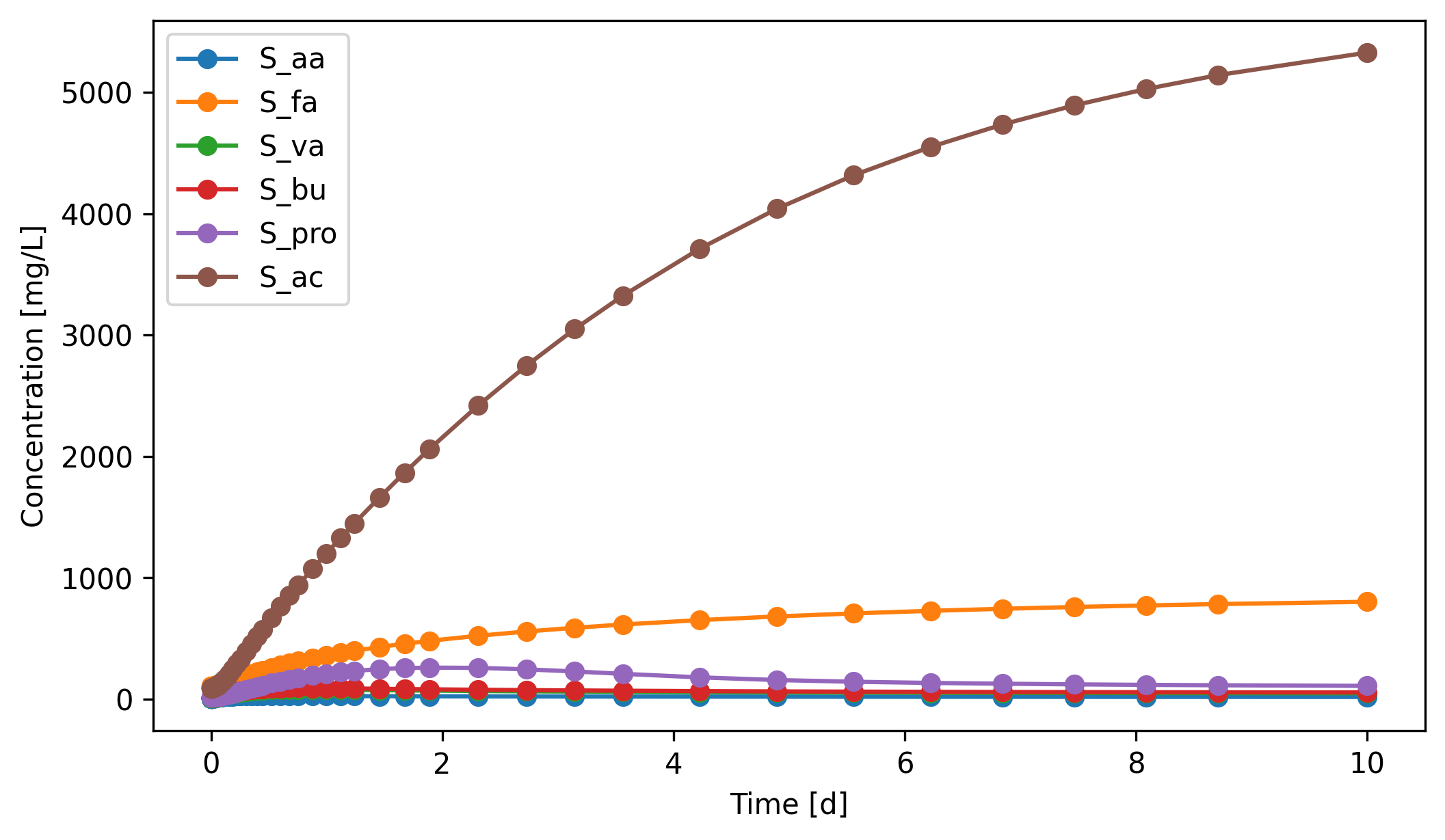
The VFA traces show three different behaviours:

• Acetate (``S_ac``) climbs from ~90 to ~5300 mg/L over the 10-day window, but the rate of accumulation slows substantially toward the end (~1100 mg/L/d around day 1 drops to ~250 mg/L/d around day 10): the curve is approaching a plateau where the high acetate concentration pushes the acetoclastic methanogens (X_ac) toward their maximum uptake rate, so methanogenesis eventually catches up with what acetogenesis releases. The plateau sits well above a healthy AD operating range (typical effluent S_ac is <100 mg/L), so the digester is still in an overloaded state.

• Long-chain fatty acids (``S_fa``) rise steadily from ~100 to ~800 mg/L. Hydrolysis of lipids produces LCFA faster than the LCFA-uptaking acetogens (X_fa) can consume them.

• Valerate (``S_va``), butyrate (``S_bu``), propionate (``S_pro``), and amino acids (``S_aa``) overshoot in the first few days then partially decline as X_c4, X_pro, and X_aa grow into the substrate pulse. S_pro peaks around ~260 mg/L near day 3 before settling toward ~110 mg/L.

This is a classic AD start-up imbalance: the upstream steps (hydrolysis, acidogenesis, acetogenesis of short VFAs) are fast, but LCFA degradation and acetoclastic methanogenesis are slow. Without intervention (lower organic load, biomass retention, longer HRT), a real digester operating in this regime would not produce a useful effluent.

# Track how each state variable changes over time
eff.scope.plot_time_series(('S_aa', 'S_fa', 'S_va', 'S_bu', 'S_pro', 'S_ac'))

(<Figure size 2400x1350 with 1 Axes>,
 <Axes: xlabel='Time [d]', ylabel='Concentration [mg/L]'>)

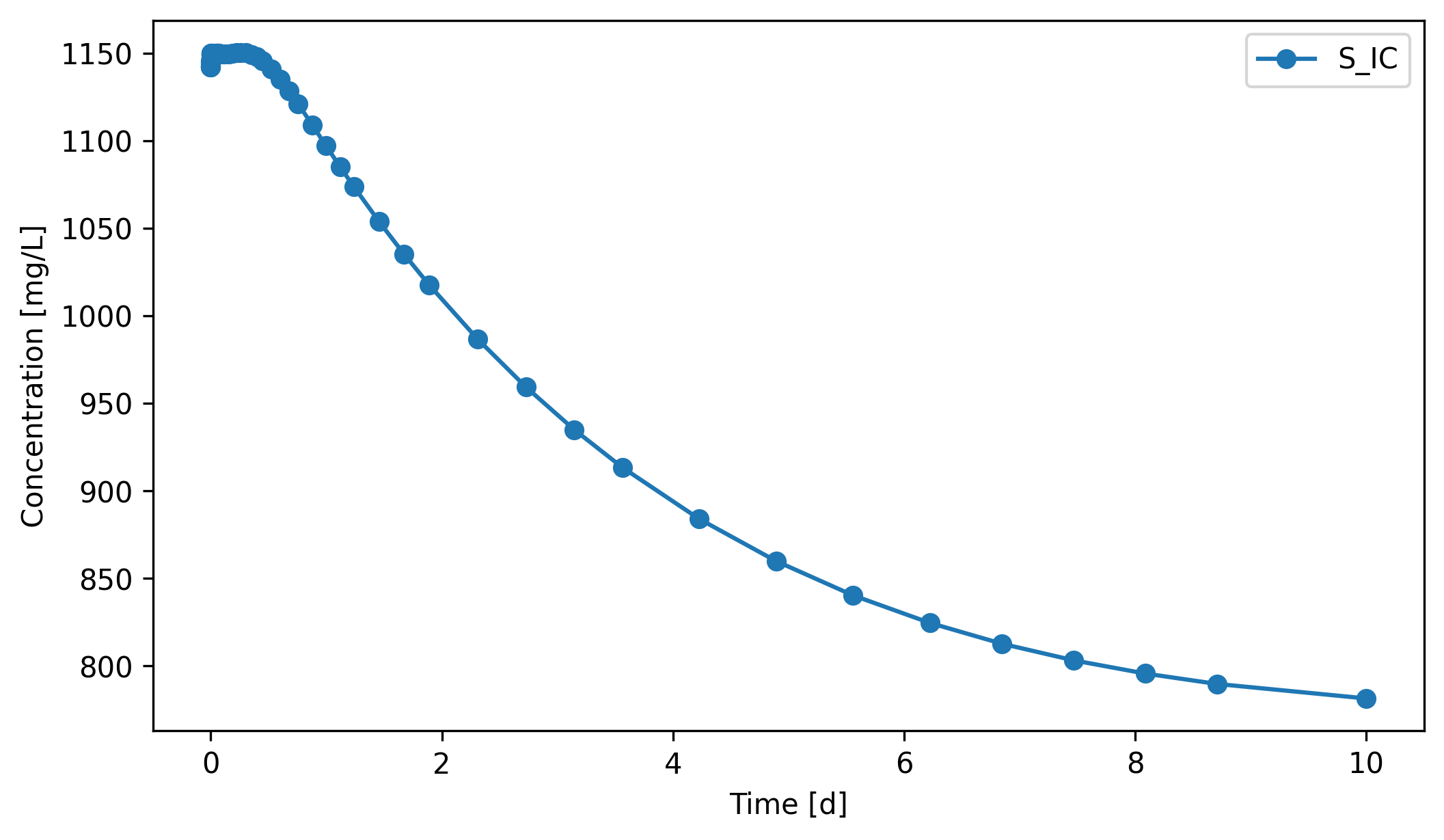
S_IC (inorganic carbon: dissolved CO₂ and HCO₃⁻) drops during this transient, from ~1140 to ~780 mg/L. The influent carries only ~480 mg/L S_IC, so at HRT = 5 d the dilution outflow pulls the liquid-phase S_IC down faster than the still-ramping-up methanogens can replenish it (acetoclastic methanogenesis is the main biological CO₂ source).

eff.scope.plot_time_series(('S_IC'))

(<Figure size 2400x1350 with 1 Axes>,
 <Axes: xlabel='Time [d]', ylabel='Concentration [mg/L]'>)

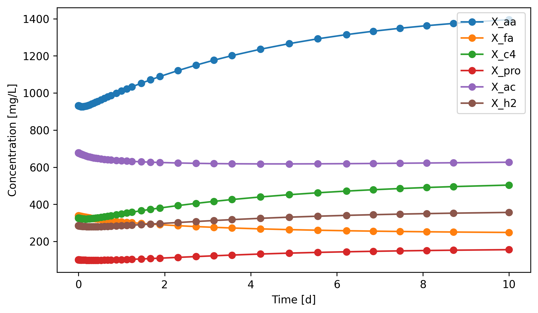
The six biomass groups split into two camps in this 10-day window:

• Growing: X_aa (+50%), X_c4 (+55%), X_pro (+54%), X_h2 (+25%). Their substrates are abundant and their net growth rate exceeds the dilution rate (1/HRT = 0.2 d⁻¹).

• Declining: X_fa (−26%) and X_ac (−7%). These two are the slowest growers in ADM1, and on top of that their net growth is reduced further by pH inhibition as VFAs accumulate. Even with plenty of substrate they can’t sustain themselves — which is exactly why S_fa and S_ac keep climbing in the plot above.

This split is the fundamental reason high-rate AD reactors decouple solids retention time (SRT) from hydraulic retention time (HRT): granular sludge, packed beds, and membrane systems all retain X_fa and X_ac against washout. See exposan.metab for examples.

eff.scope.plot_time_series(('X_aa', 'X_fa', 'X_c4', 'X_pro', 'X_ac', 'X_h2'))

(<Figure size 2400x1350 with 1 Axes>,
 <Axes: xlabel='Time [d]', ylabel='Concentration [mg/L]'>)

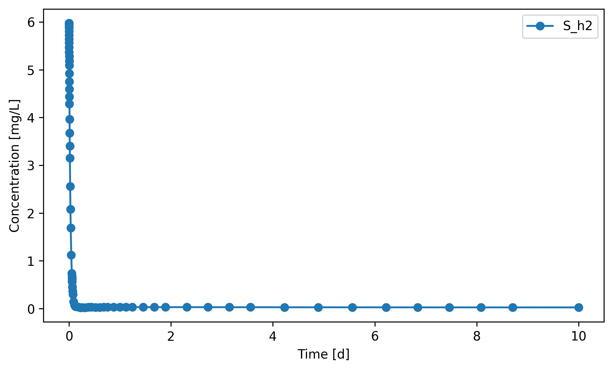
3.2. Gas

Headspace H₂ significantly decreased within the first day or two (the initial value reflects the default headspace initialisation, not a steady state) and then stays at very low partial pressures throughout the rest of the window. The hydrogenotrophic methanogens (X_h2) consume H₂ about as fast as it’s produced, and the resulting low p_H2 (< 1 mbar) is thermodynamically required for the upstream acetogenic steps — propionate and butyrate degradation are only exergonic at very low p_H2. X_h2 grows steadily through this window (+25%), confirming the tight coupling.

gas.scope.plot_time_series(('S_h2'))

(<Figure size 2400x1350 with 1 Axes>,
 <Axes: xlabel='Time [d]', ylabel='Concentration [mg/L]'>)

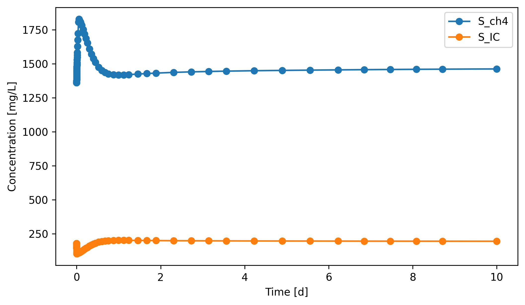
Headspace methane rises sharply in the first few days, peaks around day 3 at ~1830 mg/L, then declines back toward ~1460 mg/L as the X_ac population thins out: the digester is producing acetate faster than it can be converted to methane (consistent with the runaway S_ac in §3.1). CO₂ in the headspace follows a similar peak-and-decline pattern at much lower concentration.

gas.scope.plot_time_series(('S_ch4','S_IC'))

(<Figure size 2400x1350 with 1 Axes>,
 <Axes: xlabel='Time [d]', ylabel='Concentration [mg/L]'>)

3.3. Extensions

Relevant contents in QSDsan:

• The validation system itself. exposan.adm packages exactly this digester as a one-call load(); its test suite (EXPOsan/tests/test_adm.py) verifies the 26 state variables and the four major biogas species against the published steady state.

• ADM1 variants. exposan.adm1_p_ext adds phosphorus to the model. exposan.metab wraps ADM1 inside granular-sludge, packed-bed, and membrane-degassing reactor variants for high-rate anaerobic treatment.

• Full-plant context. exposan.bsm2 is the BSM2 benchmark: a full wastewater treatment plant where an ADM1 digester sits downstream of an activated-sludge process, with recycle loops, sludge thickeners, and so on. exposan.werf bundles seven WERF flowsheet variants (B1, C1, F1, G1, H1, I1, N1) where an AnaerobicCSTR running ADM1p (the phosphorus-extended variant) digests waste sludge from an mASM2d activated-sludge process, with ASM↔ADM interface units handling the component translation.

• Parameter studies. The uncertainty and sensitivity patterns from Tutorial 9 apply directly: you can wrap the sys here in a qs.Model, sample over ADM1 parameters (adm1.set_parameters(...)) or operating conditions (T, HRT, influent composition), and propagate through to biogas yield and effluent VFAs.

---

↑ Back to top