Process Modeling 101¶
Click the badge below to try this tutorial interactively in your browser:
![]()
You can also run this tutorial inGoogle Colab. It takes a one-time setup per session: follow theColab instructions.
Prepared by:
Learning objectives. After this tutorial, you will be able to:
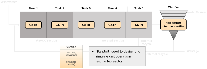
Assemble a multi-unit dynamic flowsheet from
CSTR,FlatBottomCircularClarifier, and internal plus external recycle streamsAttach a biokinetic model (
ASM2d) and a per-zone aeration model to dynamic reactorsInitialize reactor states from a file with
batch_init, run the simulation, and interpret the resulting state-variable trajectories
Prerequisites:
Covered topics:
Introduction
System setup
System simulation
Setup¶
Import QSDsan and confirm the installed version.
[1]:
import qsdsan as qs
print(f'This tutorial was made with qsdsan v{qs.__version__}.')
This tutorial was made with qsdsan v1.5.3.
1. Introduction¶
In Tutorials 10-12, we covered the building blocks of process modeling: how a kinetic model is represented (Tutorial 10 introduced the Process / CompiledProcesses classes and the Petersen / Gujer matrix), how a single dynamic unit is set up and integrated through time (Tutorial 11), and how a full biokinetic model lives inside one
reactor (Tutorial 12 uses ADM1 inside an AnaerobicCSTR).
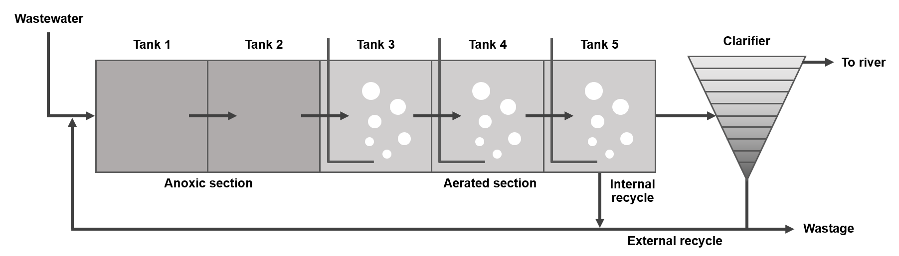
This tutorial serves both as a review and a practical application example. It puts those pieces together at the flowsheet scale: a complete A2O (anaerobic-anoxic-oxic) biological nutrient removal plant, built from five coupled dynamic CSTRs with per-zone aeration, a layered final clarifier, and internal plus external recycle streams. The biokinetic model is Activated Sludge Model No. 2d (ASM2d), the IWA-validated activated-sludge model that resolves carbon, nitrogen, and phosphorus dynamics simultaneously.
If you want to revisit the conceptual basics (components, stoichiometry, kinetics, the Petersen / Gujer matrix), Tutorial 10 and Tutorial 12 §1 cover them in depth.
2. System setup¶
2.1. Component¶
Components were defined conceptually in Tutorial 2. Here, instead of constructing each one by one, we use the precompiled ASM2d component set shipped with QSDsan.

[2]:
# Import packages
import numpy as np, pandas as pd
from qsdsan import unit_operations as su, process_models as pc, WasteStream, System
from qsdsan.utils import time_printer, load_data, get_SRT
[3]:
# Components
cmps = pc.create_asm2d_cmps()           # create components of ASM2d
                                        # you don't need to define each component one by one.
                                        # compiled components for ASM2d are already available.

cmps.show()                             # 18 components of ASM2d + water (X_TSS was excluded due to redundancy.)
CompiledComponents([
    S_O2,   S_N2,  S_NH4, S_NO3,
    S_PO4,  S_F,   S_A,   S_I,
    S_ALK,  X_I,   X_S,   X_H,
    X_PAO,  X_PP,  X_PHA, X_AUT,
    X_MeOH, X_MeP, H2O,
])
S_O2: Dissolved oxygen
S_N2: Dinitrogen
S_NH4: Ammonium plus ammonia nitrogen
S_NO3: Nitrate plus nitrite nitrogen (NO3-N + NO2-N)
S_PO4: Inorganic soluble phosphorus, primarily orthophosphates
S_F: Fermentable, readily biodegradable organic substrates
S_A: Fermentation products, considered to be acetate
S_I: Inert soluble organic material
S_ALK: Alkalinity of the wastewater
X_I: Inert particulate organic material
X_S: Slowly biodegradable substrates
X_H: Heterotrophic organisms
X_PAO: Phosphate-accumulating organisms (PAO)
X_PP: Poly-phosphate
X_PHA: A cell-internal storage product of PAO
X_AUT: Nitrifying organisms
X_MeOH: Metal-hydroxides
X_MeP: Metal-phosphate (MePO4)
[4]:
cmps.S_A.show(chemical_info=True) # each component stores thermodynamic properties.
Component: S_A (phase_ref='l')
[Names]  CAS: 71-50-1
         InChI: C2H4O2/c1-2(3)4/h1H3...
         InChI_key: QTBSBXVTEAMEQO-U...
         common_name: acetate ion
         iupac_name: ('acetate',)
         pubchemid: 175
         smiles: CC(=O)[O-]
         formula: C2H3O2-
[Groups] Dortmund: <Empty>
         UNIFAC: <Empty>
         PSRK: <Empty>
         NIST: <Empty>
[Data]   MW: 63.998 g/mol
         Tm: None
         Tb: 626.15 K
         Tt: None
         Tc: None
         Pt: None
         Pc: None
         Vc: 0.00016858 m^3/mol
         Hf: 0 J/mol
         S0: 0 J/K/mol
         LHV: 0 J/mol
         HHV: 0 J/mol
         Hfus: 0 J/mol
         Sfus: 0
         omega: None
         dipole: None
         similarity_variable: 0.11856
         iscyclic_aliphatic: 0
         combustion: {'CO2': 2, 'O2'...
Component-specific properties:
[Others] measured_as: COD
         description: Acetate
         particle_size: Soluble
         degradability: Readily
         organic: True
         i_C: 0.37535 g C/g COD
         i_N: 0 g N/g COD
         i_P: 0 g P/g COD
         i_K: 0 g K/g COD
         i_Mg: 0 g Mg/g COD
         i_Ca: 0 g Ca/g COD
         i_mass: 0.9226 g mass/g COD
         i_charge: -0.015626 mol +/g COD
         i_COD: 1 g COD/g COD
         i_NOD: 0 g NOD/g COD
         f_BOD5_COD: 0.717
         f_uBOD_COD: 0.8628
         f_Vmass_Totmass: 1
         chem_MW: 59.044
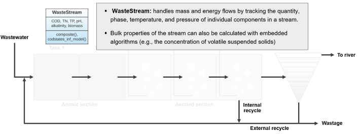
2.2. WasteStream¶
WasteStream was introduced in Tutorial 3. Here we create the influent, effluent, and recycle streams as empty WasteStream objects, then set the influent composition by concentration.
[5]:
# Parameters (flowrates, temperature)
Q_inf = 18446                               # influent flowrate [m3/d]
Q_was = 385                                 # sludge wastage flowrate [m3/d]
Q_ext = 18446                               # external recycle flowrate [m3/d]
                                            # internal recycle flowrate will be defined later using split ratio.
                                            # effluent flowrate will be calculated as the amount remaining after recycling and wastage.

Temp = 273.15+20                            # temperature [K]
[6]:
# Create influent, effluent, recycle stream
influent = WasteStream('influent', T=Temp)                         # create an empty wastestream with specified temperature
effluent = WasteStream('effluent', T=Temp)

int_recycle = WasteStream('internal_recycle', T=Temp)
ext_recycle = WasteStream('external_recycle', T=Temp)
wastage = WasteStream('wastage', T=Temp)                           # streams between the reactors will be
                                                                   # automatically assigned when we define SanUnit.
[7]:
# Set the influent composition
default_inf_kwargs = {                                             # default influent composition
    'concentrations': {                                            # you can set concentration of each component separately.
      'S_I': 14,
      'X_I': 26.5,
      'S_F': 20.1,
      'S_A': 94.3,
      'X_S': 409.75,
      'S_NH4': 31,
      'S_N2': 0,
      'S_NO3': 0.266,
      'S_PO4': 2.8,
      'X_PP': 0.05,
      'X_PHA': 0.5,
      'X_H': 0.15,
      'X_AUT': 0,
      'X_PAO': 0,
      'S_ALK':7*12,
      },
    'units': ('m3/d', 'mg/L'),                                     # ('input total flowrate', 'input concentrations')
    }

influent.set_flow_by_concentration(Q_inf, **default_inf_kwargs)    # set flowrate and composition of empty influent WasteStream
[8]:
# Wastestream stores bulk properties of the stream, as well as concentration of each component.
influent.show()
WasteStream: influent
phase: 'l', T: 293.15 K, P: 101325 Pa
flow (g/hr): S_NH4  2.38e+04
             S_NO3  204
             S_PO4  2.15e+03
             S_F    1.54e+04
             S_A    7.25e+04
             S_I    1.08e+04
             S_ALK  6.46e+04
             X_I    2.04e+04
             X_S    3.15e+05
             X_H    115
             X_PP   38.4
             X_PHA  384
             H2O    7.66e+08
 WasteStream-specific properties:
  pH         : 7.0
  Alkalinity : 2.5 mmol/L
  COD        : 565.3 mg/L
  BOD        : 320.1 mg/L
  TC         : 271.4 mg/L
  TOC        : 187.4 mg/L
  TN         : 48.9 mg/L
  TP         : 7.4 mg/L
  TK         : 0.1 mg/L
  TSS        : 327.8 mg/L
 Component concentrations (mg/L):
  S_NH4   31.0
  S_NO3   0.3
  S_PO4   2.8
  S_F     20.1
  S_A     94.3
  S_I     14.0
  S_ALK   84.0
  X_I     26.5
  X_S     409.8
  X_H     0.2
  X_PP    0.1
  X_PHA   0.5
  H2O     997254.9
[9]:
influent.get_VSS() # you can also retrieve other information, such as VSS, TSS, TDS, etc.
[9]:
324.98437505925017
2.3. Process¶
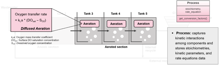
Process was covered in depth in Tutorial 10. In this tutorial we use the precompiled ASM2d biokinetic processes together with a DiffusedAeration process attached to each aerated zone to model oxygen mass transfer.
2.3.1. Aeration¶
[10]:
# Parameters (volumes)
V_an = 1000                                 # anoxic zone tank volume [m3/d]
V_ae = 1333                                 # aerated zone tank volume [m3/d]
[11]:
# Aeration model
aer1 = pc.DiffusedAeration('aer1', DO_ID='S_O2', KLa=240, DOsat=8.0, V=V_ae)             # aeration model for Tank 3 & Tank 4
aer2 = pc.DiffusedAeration('aer2', DO_ID='S_O2', KLa=84, DOsat=8.0, V=V_ae)              # aeration model for Tank 5
DO_ID: The component ID of dissolved oxygen (DO).
KLa: Oxygen mass transfer coefficient.
DOsat: Surface DO saturation concentration.
V: Reactor volume
[12]:
aer1.show()
Process: aer1
[stoichiometry]      S_O2: 1
[reference]          S_O2
[rate equation]      KLa*(DOsat - S_O2)
[parameters]         KLa: 240
                     DOsat: 8
[dynamic parameters]
2.3.2. ASM2d¶
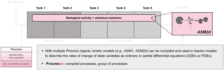
[13]:
# ASM2d
asm2d = pc.ASM2d()                       # create ASM2d processes
asm2d.show()                             # 21 processes in ASM2d
ASM2d([aero_hydrolysis, anox_hydrolysis, anae_hydrolysis, hetero_growth_S_F, hetero_growth_S_A, denitri_S_F, denitri_S_A, ferment, hetero_lysis, PAO_storage_PHA, aero_storage_PP, anox_storage_PP, PAO_aero_growth_PHA, PAO_anox_growth, PAO_lysis, PP_lysis, PHA_lysis, auto_aero_growth, auto_lysis, precipitation, redissolution])
[14]:
asm2d.aero_hydrolysis # Each process includes stoichiometry, rate equation, and parameters.
Process: aero_hydrolysis
[stoichiometry]      S_NH4: 0.02*f_SI + 0.01
                     S_PO4: 0.01*f_SI
                     S_F: 1.0 - 1.0*f_SI
                     S_I: 1.0*f_SI
                     S_ALK: 0.0113*f_SI + 0.00858
                     X_S: -1.00
[reference]          X_S
[rate equation]      K_h*S_O2*X_S/((K_O2 + S_O2)*...
[parameters]         f_SI: 0
                     Y_H: 0.625
                     f_XI_H: 0.1
                     Y_PAO: 0.625
                     Y_PO4: 0.4
                     Y_PHA: 0.2
                     f_XI_PAO: 0.1
                     Y_A: 0.24
                     f_XI_AUT: 0.1
                     K_h: 3
                     eta_NO3: 0.6
                     eta_fe: 0.4
                     K_O2: 0.2
                     K_NO3: 0.5
                     K_X: 0.1
                     mu_H: 6
                     q_fe: 3
                     eta_NO3_H: 0.8
                     b_H: 0.4
                     K_O2_H: 0.2
                     K_F: 4
                     K_fe: 4
                     K_A_H: 4
                     K_NO3_H: 0.5
                     K_NH4_H: 0.05
                     K_P_H: 0.01
                     K_ALK_H: 1.2
                     q_PHA: 3
                     q_PP: 1.5
                     mu_PAO: 1
                     eta_NO3_PAO: 0.6
                     b_PAO: 0.2
                     b_PP: 0.2
                     b_PHA: 0.2
                     K_O2_PAO: 0.2
                     K_NO3_PAO: 0.5
                     K_A_PAO: 4
                     K_NH4_PAO: 0.05
                     K_PS: 0.2
                     K_P_PAO: 0.01
                     K_ALK_PAO: 1.2
                     K_PP: 0.01
                     K_MAX: 0.34
                     K_IPP: 0.02
                     K_PHA: 0.01
                     mu_AUT: 1
                     b_AUT: 0.15
                     K_O2_AUT: 0.5
                     K_NH4_AUT: 1
                     K_ALK_AUT: 6
                     K_P_AUT: 0.01
                     k_PRE: 1
                     k_RED: 0.6
                     K_ALK_PRE: 6
                     COD_deN: 2.86
[dynamic parameters]
[15]:
# Petersen stoichiometric matrix of ASM2d
pd.set_option('display.max_columns', None)                  # to display all columns

asm2d.stoichiometry
[15]:
| S_O2 | S_N2 | S_NH4 | S_NO3 | S_PO4 | S_F | S_A | S_I | S_ALK | X_I | X_S | X_H | X_PAO | X_PP | X_PHA | X_AUT | X_MeOH | X_MeP | H2O | |
|---|---|---|---|---|---|---|---|---|---|---|---|---|---|---|---|---|---|---|---|
| aero_hydrolysis | 0 | 0 | 0.01 | 0 | 0 | 1 | 0 | 0 | 0.00857 | 0 | -1 | 0 | 0 | 0 | 0 | 0 | 0 | 0 | 0 |
| anox_hydrolysis | 0 | 0 | 0.01 | 0 | 0 | 1 | 0 | 0 | 0.00857 | 0 | -1 | 0 | 0 | 0 | 0 | 0 | 0 | 0 | 0 |
| anae_hydrolysis | 0 | 0 | 0.01 | 0 | 0 | 1 | 0 | 0 | 0.00857 | 0 | -1 | 0 | 0 | 0 | 0 | 0 | 0 | 0 | 0 |
| hetero_growth_S_F | -0.6 | 0 | -0.022 | 0 | -0.004 | -1.6 | 0 | 0 | -0.0165 | 0 | 0 | 1 | 0 | 0 | 0 | 0 | 0 | 0 | 0 |
| hetero_growth_S_A | -0.6 | 0 | -0.07 | 0 | -0.02 | 0 | -1.6 | 0 | 0.252 | 0 | 0 | 1 | 0 | 0 | 0 | 0 | 0 | 0 | 0 |
| denitri_S_F | 0 | 0.21 | -0.022 | -0.21 | -0.004 | -1.6 | 0 | 0 | 0.164 | 0 | 0 | 1 | 0 | 0 | 0 | 0 | 0 | 0 | 0 |
| denitri_S_A | 0 | 0.21 | -0.07 | -0.21 | -0.02 | 0 | -1.6 | 0 | 0.432 | 0 | 0 | 1 | 0 | 0 | 0 | 0 | 0 | 0 | 0 |
| ferment | 0 | 0 | 0.03 | 0 | 0.01 | -1 | 1 | 0 | -0.168 | 0 | 0 | 0 | 0 | 0 | 0 | 0 | 0 | 0 | 0 |
| hetero_lysis | 0 | 0 | 0.032 | 0 | 0.01 | 0 | 0 | 0 | 0.0216 | 0.1 | 0.9 | -1 | 0 | 0 | 0 | 0 | 0 | 0 | 0 |
| PAO_storage_PHA | 0 | 0 | 0 | 0 | 0.4 | 0 | -1 | 0 | 0.11 | 0 | 0 | 0 | 0 | -0.4 | 1 | 0 | 0 | 0 | 0 |
| aero_storage_PP | -0.2 | 0 | 0 | 0 | -1 | 0 | 0 | 0 | 0.194 | 0 | 0 | 0 | 0 | 1 | -0.2 | 0 | 0 | 0 | 0 |
| anox_storage_PP | 0 | 0.07 | -7.78e-18 | -0.07 | -1 | 0 | 0 | 0 | 0.254 | 0 | 0 | 0 | 0 | 1 | -0.2 | 0 | 0 | 0 | 0 |
| PAO_aero_growth_PHA | -0.6 | 0 | -0.07 | 0 | -0.02 | 0 | 0 | 0 | -0.0484 | 0 | 0 | 0 | 1 | 0 | -1.6 | 0 | 0 | 0 | 0 |
| PAO_anox_growth | 0 | 0.21 | -0.07 | -0.21 | -0.02 | 0 | 0 | 0 | 0.132 | 0 | 0 | 0 | 1 | 0 | -1.6 | 0 | 0 | 0 | 0 |
| PAO_lysis | 0 | 0 | 0.032 | 0 | 0.01 | 0 | 0 | 0 | 0.0216 | 0.1 | 0.9 | 0 | -1 | 0 | 0 | 0 | 0 | 0 | 0 |
| PP_lysis | 0 | 0 | 0 | 0 | 1 | 0 | 0 | 0 | -0.194 | 0 | 0 | 0 | 0 | -1 | 0 | 0 | 0 | 0 | 0 |
| PHA_lysis | 0 | 0 | 0 | 0 | 0 | 0 | 1 | 0 | -0.188 | 0 | 0 | 0 | 0 | 0 | -1 | 0 | 0 | 0 | 0 |
| auto_aero_growth | -18 | 0 | -4.24 | 4.17 | -0.02 | 0 | 0 | 0 | -7.19 | 0 | 0 | 0 | 0 | 0 | 0 | 1 | 0 | 0 | 0 |
| auto_lysis | 0 | 0 | 0.032 | 0 | 0.01 | 0 | 0 | 0 | 0.0216 | 0.1 | 0.9 | 0 | 0 | 0 | 0 | -1 | 0 | 0 | 0 |
| precipitation | 0 | 0 | 0 | 0 | -1 | 0 | 0 | 0 | 0.582 | 0 | 0 | 0 | 0 | 0 | 0 | 0 | -3.45 | 4.87 | 0 |
| redissolution | 0 | 0 | 0 | 0 | 1 | 0 | 0 | 0 | -0.582 | 0 | 0 | 0 | 0 | 0 | 0 | 0 | 3.45 | -4.87 | 0 |
[16]:
# Rate equations of ASM2d
asm2d.rate_equations
[16]:
| rate_equation | |
|---|---|
| aero_hydrolysis | 3.0*S_O2*X_S/((0.1 + X_S/X_H)*(... |
| anox_hydrolysis | 0.36*S_NO3*X_S/((0.1 + X_S/X_H)... |
| anae_hydrolysis | 0.12*X_S/((0.1 + X_S/X_H)*(S_NO... |
| hetero_growth_S_F | 6.0*S_ALK*S_F**2*S_NH4*S_O2*S_P... |
| hetero_growth_S_A | 6.0*S_A**2*S_ALK*S_NH4*S_O2*S_P... |
| denitri_S_F | 0.96*S_ALK*S_F**2*S_NH4*S_NO3*S... |
| denitri_S_A | 0.96*S_A**2*S_ALK*S_NH4*S_NO3*S... |
| ferment | 0.3*S_ALK*S_F*X_H/((S_ALK + 1.2... |
| hetero_lysis | 0.4*X_H |
| PAO_storage_PHA | 3.0*S_A*S_ALK*X_PP/((0.01 + X_P... |
| aero_storage_PP | 1.5*S_ALK*S_O2*S_PO4*X_PHA*(0.3... |
| anox_storage_PP | 0.18*S_ALK*S_NO3*S_PO4*X_PHA*(0... |
| PAO_aero_growth_PHA | 1.0*S_ALK*S_NH4*S_O2*S_PO4*X_PH... |
| PAO_anox_growth | 0.12*S_ALK*S_NH4*S_NO3*S_PO4*X_... |
| PAO_lysis | 0.2*S_ALK*X_PAO/(S_ALK + 1.2) |
| PP_lysis | 0.2*S_ALK*X_PP/(S_ALK + 1.2) |
| PHA_lysis | 0.2*S_ALK*X_PHA/(S_ALK + 1.2) |
| auto_aero_growth | 1.0*S_ALK*S_NH4*S_O2*S_PO4*X_AU... |
| auto_lysis | 0.15*X_AUT |
| precipitation | 1.0*S_PO4*X_MeOH |
| redissolution | 0.6*S_ALK*X_MeP/(S_ALK + 6.0) |
2.4. SanUnit¶
Static SanUnits were introduced in Tutorial 4 and Tutorial 5; a single dynamic unit was the focus of Tutorial 11. Here we assemble five dynamic CSTRs, each carrying both an aeration and a suspended-growth biokinetic model, plus a 10-layer
FlatBottomCircularClarifier for final settling.
[17]:
# Anoxic reactors (Tank 1 & Tank 2)
A1 = su.CSTR('A1', ins=[influent, int_recycle, ext_recycle], V_max=V_an,      # As CSTR, 3 input streams, tank volume as V_an
             aeration=None, suspended_growth_model=asm2d)                     # No aeration, biokinetic model as asm2d

A2 = su.CSTR('A2', ins=A1-0, V_max=V_an,                 # ins=A1-0: set influent of A2 as effluent of A1 reactor (to connect A1 with A2)
             aeration=None, suspended_growth_model=asm2d)
ins: influents to the reactor.
outs: treated effluent from the reactor.
V_max: designed reactor volume [m^3].
aeration: aeration setting: a target dissolved oxygen concentration [mg O2/L], a
Processobject representing - aeration, orNonefor no aeration.suspended_growth_model: the suspended-growth biokinetic model.
See the CSTR documentation for the full signature and default values (you can also run ?su.CSTR in IPython).
[18]:
# Before simulation, outs are empty.
A1.show()
CSTR: A1
ins...
[0] influent
phase: 'l', T: 293.15 K, P: 101325 Pa
flow (g/hr): S_NH4  2.38e+04
                S_NO3  204
                S_PO4  2.15e+03
                S_F    1.54e+04
                S_A    7.25e+04
                S_I    1.08e+04
                S_ALK  6.46e+04
                X_I    2.04e+04
                X_S    3.15e+05
                X_H    115
                X_PP   38.4
                X_PHA  384
                H2O    7.66e+08
    WasteStream-specific properties:
     pH         : 7.0
     Alkalinity : 2.5 mmol/L
     COD        : 565.3 mg/L
     BOD        : 320.1 mg/L
     TC         : 271.4 mg/L
     TOC        : 187.4 mg/L
     TN         : 48.9 mg/L
     TP         : 7.4 mg/L
     TK         : 0.1 mg/L
     TSS        : 327.8 mg/L
[1] internal_recycle
phase: 'l', T: 293.15 K, P: 101325 Pa
flow: 0
    WasteStream-specific properties: None for empty waste streams
[2] external_recycle
phase: 'l', T: 293.15 K, P: 101325 Pa
flow: 0
    WasteStream-specific properties: None for empty waste streams
outs...
[0] ws1  to  CSTR-A2
phase: 'l', T: 298.15 K, P: 101325 Pa
flow: 0
    WasteStream-specific properties: None for empty waste streams
[19]:
# Aerated reactors (Tank 3, Tank 4, Tank 5)
O1 = su.CSTR('O1', ins=A2-0, V_max=V_ae, aeration=aer1,                          # tank volume as V_ae with aeration model1
             DO_ID='S_O2', suspended_growth_model=asm2d)

O2 = su.CSTR('O2', ins=O1-0, V_max=V_ae, aeration=aer1,
             DO_ID='S_O2', suspended_growth_model=asm2d)

O3 = su.CSTR('O3', ins=O2-0, outs=[int_recycle, 'treated'], split=[0.6, 0.4],    # 60% of effluent to internal recycle, 40% to clarifier
             V_max=V_ae, aeration=aer2,
             DO_ID='S_O2', suspended_growth_model=asm2d)
[20]:
O3.show()
CSTR: O3
ins...
[0] ws7  from  CSTR-O2
phase: 'l', T: 298.15 K, P: 101325 Pa
flow: 0
    WasteStream-specific properties: None for empty waste streams
outs...
[0] internal_recycle  to  CSTR-A1
phase: 'l', T: 293.15 K, P: 101325 Pa
flow: 0
    WasteStream-specific properties: None for empty waste streams
[1] treated
phase: 'l', T: 298.15 K, P: 101325 Pa
flow: 0
    WasteStream-specific properties: None for empty waste streams
[21]:
# Clarifier
C1 = su.FlatBottomCircularClarifier('C1', ins=O3-1, outs=[effluent, ext_recycle, wastage],  # O3-1: second effluent of O3, three outs
                                    underflow=Q_ext, wastage=Q_was, surface_area=1500,
                                    height=4, N_layer=10, feed_layer=5,                     # modeled as a 10 layer non-reactive unit
                                    X_threshold=3000, v_max=474, v_max_practical=250,
                                    rh=5.76e-4, rp=2.86e-3, fns=2.28e-3)
underflow: designed recycling sludge flowrate (RAS) [m^3/d].
wastage: designed wasted sludge flowrate (WAS) [m^3/d].
surface_area: surface area of the clarifier [m^2].
height: height of the clarifier [m].
N_layer: number of layers used to model settling.
feed_layer: the feed layer, counted from the top.
X_threshold: threshold suspended-solids concentration [g/m^3].
v_max: maximum theoretical (Vesilind) settling velocity [m/d].
v_max_practical: maximum practical settling velocity [m/d].
rh: hindered-zone settling parameter in the double-exponential settling-velocity function [m^3/g].
rp: flocculant-zone settling parameter in the double-exponential settling-velocity function [m^3/g].
fns: non-settleable fraction of the suspended solids (dimensionless, within [0, 1]).
See the FlatBottomCircularClarifier documentation for the full signature and default values (you can also run ?su.FlatBottomCircularClarifier in IPython).
2.5. System¶
Static System assembly was introduced in Tutorial 6; single-unit dynamic simulation in Tutorial 11. Here we assemble a multi-unit flowsheet with internal plus external recycle streams, set per-reactor initial conditions through batch_init, and let the System organize unit operations for mass-balance convergence, techno-economic
analysis (TEA), and life cycle assessment (LCA).

2.5.1. Create system¶
[22]:
# Create system
sys = System('example_system', path=(A1, A2, O1, O2, O3, C1), recycle=(int_recycle, ext_recycle))     # path: the order of reactor
[23]:
# System diagram
sys.diagram()

2.5.2. Set initial conditions of reactors¶
[24]:
# Import initial condition excel file
df = load_data('assets/tutorial_13/initial_conditions_asm2d.xlsx', sheet='default')
[25]:
df # Unlike other reactors, C1 has 3 rows for each of soluble, solids, and tss.
[25]:
| S_O2 | S_NH4 | S_NO3 | S_PO4 | S_F | S_A | S_I | S_ALK | X_I | X_S | X_H | X_PAO | X_PP | X_PHA | X_AUT | |
|---|---|---|---|---|---|---|---|---|---|---|---|---|---|---|---|
| A1 | 0.00213 | 7.23 | 10.2 | 4.45 | 0.211 | 0.0265 | 15.9 | 67 | 2.28e+03 | 84.4 | 3.78e+03 | 322 | 37.2 | 0.0517 | 218 |
| A2 | 0.001 | 22.4 | 2.4 | 4.24 | 6.68 | 53.8 | 14.5 | 79 | 0 | 84.1 | 207 | 18.2 | 4.25 | 3.59 | 11.9 |
| O2 | 2 | 16.5 | 4.31 | 5.48 | 1.9 | 2.73 | 13.7 | 82.6 | 611 | 77.3 | 1.04e+03 | 86.4 | 6.45 | 11 | 58 |
| O3 | 2 | 10.9 | 9.31 | 2.62 | 0.649 | 0.163 | 14.1 | 74.2 | 662 | 59.3 | 1.14e+03 | 95.7 | 9.99 | 7.24 | 64 |
| O1 | 2 | 0.111 | 26.1 | 2.32 | 0.276 | 0.00407 | 18.2 | 46.1 | 2.24e+03 | 61.1 | 3.79e+03 | 322 | 38.4 | 0.00852 | 218 |
| C1_s | 2 | 0.114 | 20.9 | 0.356 | 0.307 | 0.00537 | 20.1 | 49.6 | NaN | NaN | NaN | NaN | NaN | NaN | NaN |
| C1_x | NaN | NaN | NaN | NaN | NaN | NaN | NaN | NaN | 2.24e+03 | 61.1 | 3.79e+03 | 322 | 38.4 | 0.00852 | 218 |
| C1_tss | 17.8 | 27.9 | 44.9 | 90.5 | 305 | 304 | 306 | 304 | 304 | 5.83e+03 | NaN | NaN | NaN | NaN | NaN |
[26]:
# Create a function to set initial conditions of the reactors
def batch_init(sys, df):
    dct = df.to_dict('index')                                         # convert the DataFrame to a dictionary.
    u = sys.flowsheet.unit                                            # unit registry (A1, A2, O1, O2, O3, C1)

    for k in [u.A1, u.A2, u.O1, u.O2, u.O3]:                          # for A1, A2, O1, O2, O3 reactor,
        k.set_init_conc(**dct[k._ID])                                 # A1.set_init_conc(**dct[k_ID])

    c1s = {k:v for k,v in dct['C1_s'].items() if v>0}                # for clarifier, need to use different methods
    c1x = {k:v for k,v in dct['C1_x'].items() if v>0}
    tss = [v for v in dct['C1_tss'].values() if v>0]
    u.C1.set_init_solubles(**c1s)                                     # set solubles
    u.C1.set_init_sludge_solids(**c1x)                                # set sludge solids
    u.C1.set_init_TSS(tss)                                            # set TSS
[27]:
# Set the initial conditions of the system
batch_init(sys, df)
3. System simulation¶
3.1. Run simulation¶
The solve_ivp loop from Tutorial 11 now drives the entire flowsheet rather than a single reactor: at each integrator step, every dynamic unit’s state derivative _dstate is evaluated and the global state vector is advanced. Because the flowsheet has two recycle loops (internal between O3 and A1, external between C1 and A1), sys.simulate repeats the full integration in an outer convergence loop until the
recycle stream compositions satisfy sys.set_tolerance(rmol=1e-6). The line after 5 loops in the system display below reports how many of those outer passes were needed.
[28]:
# Simulation settings
sys.set_dynamic_tracker(influent, effluent, A1, A2, O1, O2, O3, C1, wastage)           # what you want to track changes in concentration
sys.set_tolerance(rmol=1e-6)

biomass_IDs = ('X_H', 'X_PAO', 'X_AUT')
[29]:
# Simulation settings
t = 50                          # total time for simulation
t_step = 1                      # times at which to store the computed solution

method = 'BDF'                  # integration method to use
# method = 'RK45'
# method = 'RK23'
# method = 'DOP853'
# method = 'Radau'
# method = 'LSODA'

# https://docs.scipy.org/doc/scipy/reference/generated/scipy.integrate.solve_ivp.html
[30]:
# Run simulation, this could take several minutes
sys.simulate(state_reset_hook='reset_cache',
             t_span=(0,t),
             t_eval=np.arange(0, t+t_step, t_step),
             method=method,
            # export_state_to=f'sol_{t}d_{method}.xlsx',               # uncomment to export simulation result as excel file
            )
[31]:
srt = get_SRT(sys, biomass_IDs)
print(f'Estimated SRT assuming at steady state is {round(srt, 2)} days')
Estimated SRT assuming at steady state is 10.02 days
The estimated solids retention time (SRT) of about 10 days matches the typical design point for a BNR plant of this size, confirming that the recycle ratios and wastage flowrate set in §2.2 produce the intended sludge inventory at quasi-steady state.
[32]:
sys.show()
System: example_system
Highest convergence error among components in recycle
streams {C1-1, O3-0} after 5 loops:
- flow rate   1.46e-11 kmol/hr (5.4e-14%)
- temperature 0.00e+00 K (0%)
ins...
[0] influent
    phase: 'l', T: 293.15 K, P: 101325 Pa
    flow (kmol/hr): S_NH4  1.7
                    S_NO3  0.0146
                    S_PO4  0.0347
                    S_F    15.4
                    S_A    1.13
                    S_I    10.8
                    S_ALK  5.38
                    ...    4.29e+04
outs...
[0] effluent
    phase: 'l', T: 293.15 K, P: 101325 Pa
    flow (kmol/hr): S_O2   0.000506
                    S_N2   0.00716
                    S_NH4  1.99
                    S_NO3  9.69e-09
                    S_PO4  0.0469
                    S_F    0.973
                    S_A    0.104
                    ...    4.17e+04
[1] wastage
    phase: 'l', T: 293.15 K, P: 101325 Pa
    flow (kmol/hr): S_O2   1.08e-05
                    S_N2   0.000153
                    S_NH4  0.0424
                    S_NO3  2.07e-10
                    S_PO4  0.000999
                    S_F    0.0207
                    S_A    0.00222
                    ...    1.04e+03
3.2. Check simulation results¶
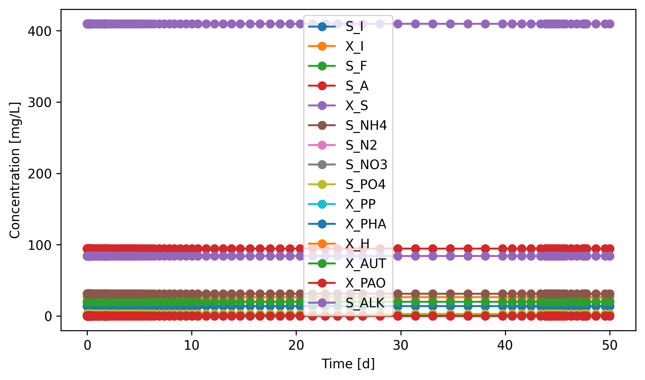
Note. The influent composition stays constant throughout this simulation (set once in §2.2 via set_flow_by_concentration), so its state-variable plot is flat. For time-varying inputs (diurnal patterns, step changes, file-driven profiles), see the DynamicInfluent walkthrough in Tutorial 11 §3.2.
[33]:
# Influent
influent.scope.plot_time_series(
    ('S_I','X_I','S_F','S_A','X_S','S_NH4','S_N2','S_NO3','S_PO4',
     'X_PP','X_PHA','X_H','X_AUT','X_PAO','S_ALK')
)
[33]:
(<Figure size 2400x1350 with 1 Axes>,
 <Axes: xlabel='Time [d]', ylabel='Concentration [mg/L]'>)
[34]:
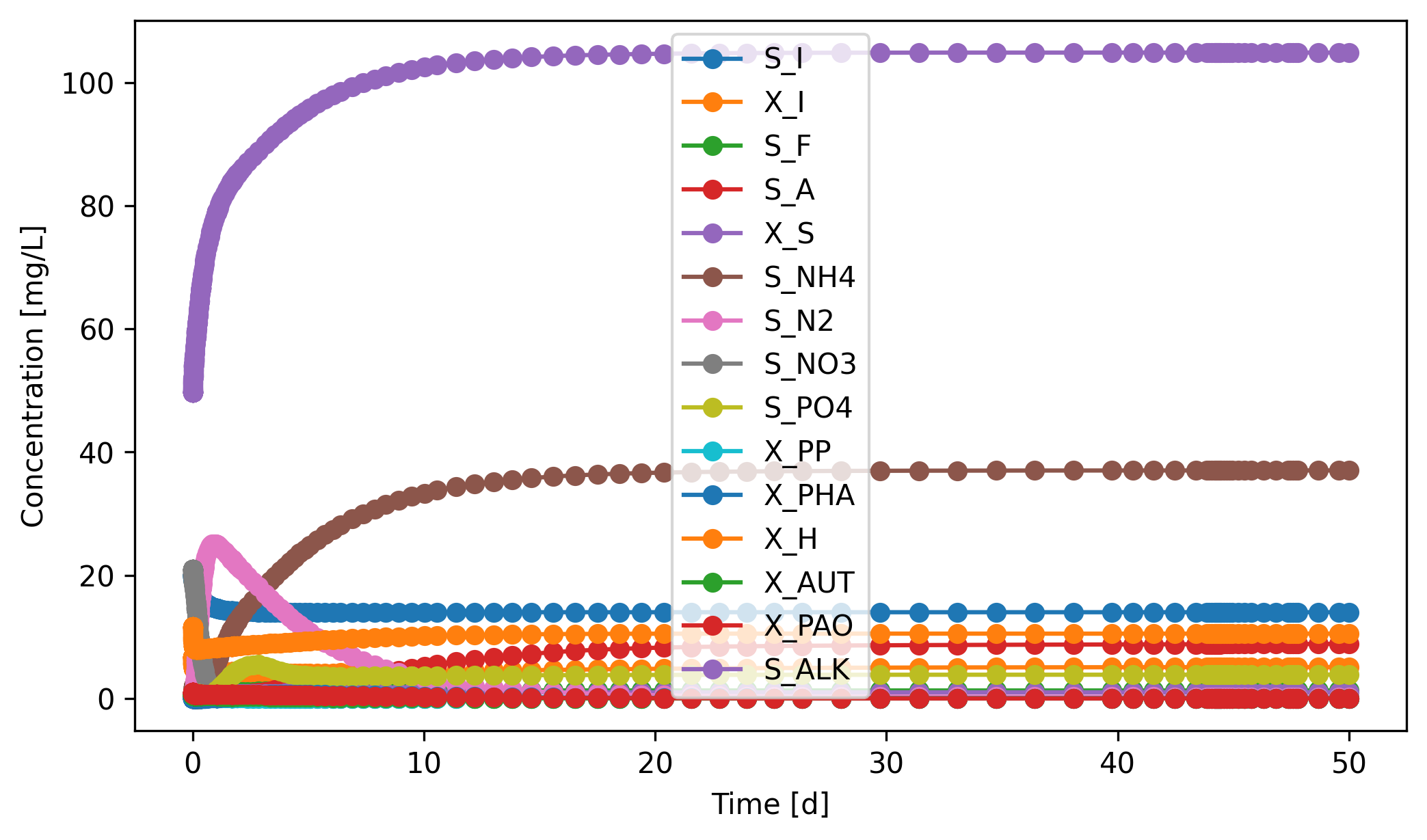
# However, the effluent does change over time, especially in the beginning of the simulation, as the system is not at steady state yet.
effluent.scope.plot_time_series((('S_I','X_I','S_F','S_A','X_S','S_NH4','S_N2','S_NO3','S_PO4','X_PP','X_PHA',
                                 'X_H','X_AUT','X_PAO','S_ALK')))                   # you can plot how each state variable changes over time
[34]:
(<Figure size 2400x1350 with 1 Axes>,
 <Axes: xlabel='Time [d]', ylabel='Concentration [mg/L]'>)
[35]:
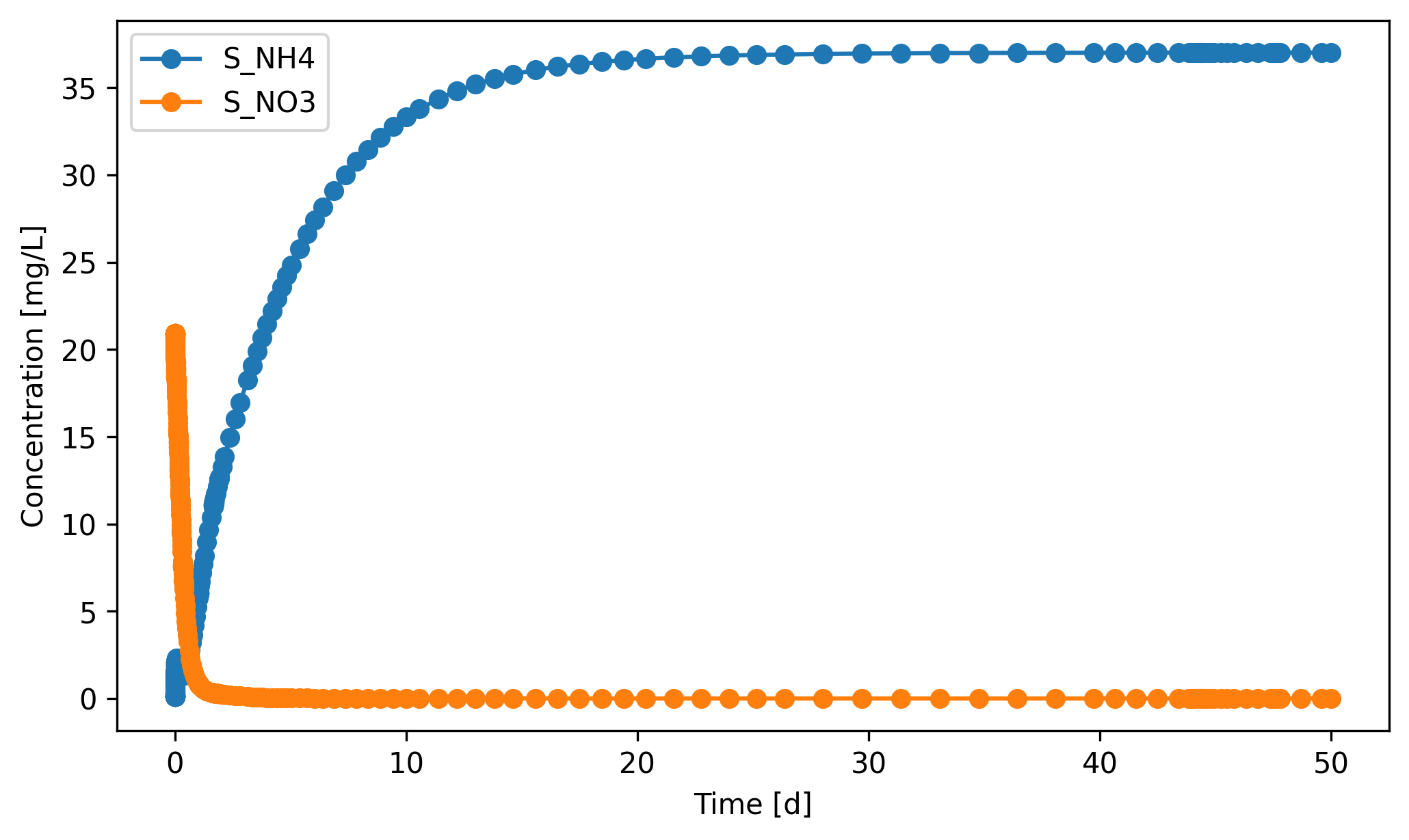
effluent.scope.plot_time_series(('S_NH4', 'S_NO3')) # you can plot how each state variable changes over time
[35]:
(<Figure size 2400x1350 with 1 Axes>,
 <Axes: xlabel='Time [d]', ylabel='Concentration [mg/L]'>)
[36]:
effluent.scope.plot_time_series(('S_O2')) # you can plot how each state variable changes over time
[36]:
(<Figure size 2400x1350 with 1 Axes>,
 <Axes: xlabel='Time [d]', ylabel='Concentration [mg/L]'>)
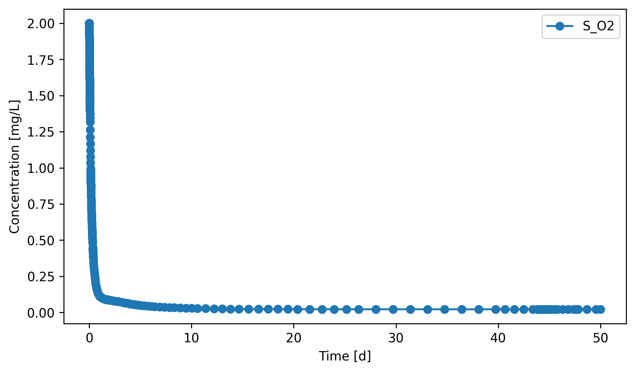
What to look for. A few features of these state trajectories are characteristic of a working BNR plant:
S_NH4 down, S_NO3 up in the effluent. Ammonium drops while nitrate rises in the aerated zones, the signature of nitrification by
X_AUT(autotrophic biomass). The remaining nitrate is either recycled internally to the anoxic zones for denitrification, or leaves with the effluent.Dissolved oxygen tracks the KLa setting. The effluent
S_O2trajectory rises to a value set by the balance between aeration supply (KLa * (DOsat - S_O2)in Tank 5, where the effluent is drawn) and biological demand. This is the same exogenous-input pattern covered in Tutorial 11 §3.1, applied per zone.Quasi-steady state by ~50 days. Because all reactors started near a representative operating point (the initial conditions in §2.5.2), the simulation reaches a near-steady state within the 50-day window. A cold-start run would take several SRT (roughly 30 to 40 days here) to wash in.
From here, you can change the influent composition, the KLa values, the recycle split, or the WAS flowrate, and re-run the simulation to see how each design parameter shifts effluent quality and SRT.
↑ Back to top